Use cases and examples
1. Examples overview
OptaPlanner has several examples. In this manual we explain mainly using the n queens example and cloud balancing example. So it is advisable to read at least those sections.
Some of the examples solve problems that are presented in academic contests.
The Contest column in the following table lists the contests.
It also identifies an example as being either realistic or unrealistic for the purpose of a contest.
A realistic contest is an official, independent contest:
-
that clearly defines a real-world use case.
-
with real-world constraints.
-
with multiple, real-world datasets.
-
that expects reproducible results within a specific time limit on specific hardware.
-
that has had serious participation from the academic and/or enterprise Operations Research community.
Realistic contests provide an objective comparison of OptaPlanner with competitive software and academic research.
The source code of all these examples is available in the distribution zip under examples/sources and also in git under optaplanner/optaplanner-examples.
| Example | Domain | Size | Contest | Special features used |
|---|---|---|---|---|
|
|
|
None |
|
|
|
|
||
|
|
|
||
|
|
|
||
|
|
|
||
|
|
|
||
|
|
|
||
|
|
|
|
|
Vehicle routing with time windows |
|
|
|
|
|
|
|
||
|
|
|
||
|
|
|
||
|
|
|
|
|
|
|
|
||
|
|
|
|
|
|
|
|
||
|
|
|
2. N queens
2.1. Problem description
Place n queens on a n sized chessboard so that no two queens can attack each other. The most common n queens puzzle is the eight queens puzzle, with n = 8:
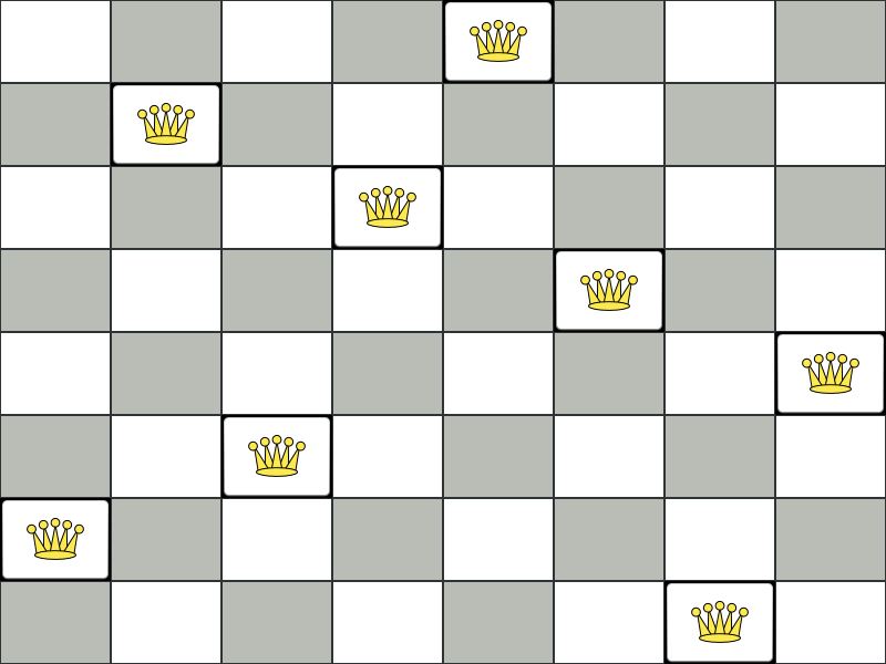
Constraints:
-
Use a chessboard of n columns and n rows.
-
Place n queens on the chessboard.
-
No two queens can attack each other. A queen can attack any other queen on the same horizontal, vertical or diagonal line.
This documentation heavily uses the four queens puzzle as the primary example.
A proposed solution could be:
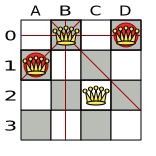
The above solution is wrong because queens A1 and B0 can attack each other (so can queens B0 and D0). Removing queen B0 would respect the "no two queens can attack each other" constraint, but would break the "place n queens" constraint.
Below is a correct solution:
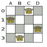
All the constraints have been met, so the solution is correct.
Note that most n queens puzzles have multiple correct solutions. We will focus on finding a single correct solution for a given n, not on finding the number of possible correct solutions for a given n.
2.2. Problem size
4queens   has   4 queens with a search space of    256.
8queens   has   8 queens with a search space of   10^7.
16queens  has  16 queens with a search space of  10^19.
32queens  has  32 queens with a search space of  10^48.
64queens  has  64 queens with a search space of 10^115.
256queens has 256 queens with a search space of 10^616.
The implementation of the n queens example has not been optimized because it functions as a beginner example. Nevertheless, it can easily handle 64 queens. With a few changes it has been shown to easily handle 5000 queens and more.
2.3. Domain model
This example uses the domain model to solve the four queens problem.
-
Creating a Domain Model A good domain model will make it easier to understand and solve your planning problem.
This is the domain model for the n queens example:
public class Column {

    private int index;

    // ... getters and setters
}
public class Row { private int index; // ... getters and setters }public class Queen { private Column column; private Row row; public int getAscendingDiagonalIndex() {...} public int getDescendingDiagonalIndex() {...} // ... getters and setters } -
Calculating the Search Space.
A
Queeninstance has aColumn(for example: 0 is column A, 1 is column B, …) and aRow(its row, for example: 0 is row 0, 1 is row 1, …).The ascending diagonal line and the descending diagonal line can be calculated based on the column and the row.
The column and row indexes start from the upper left corner of the chessboard.
public class NQueens { private int n; private List<Column> columnList; private List<Row> rowList; private List<Queen> queenList; private SimpleScore score; // ... getters and setters } -
Finding the Solution
A single
NQueensinstance contains a list of allQueeninstances. It is the solution implementation which is supplied to, solved by, and retrieved from theSolver.
Notice that in the four queens example, NQueens’s getN() method will always return four.
| A solution | Queen | columnIndex | rowIndex | ascendingDiagonalIndex (columnIndex + rowIndex) | descendingDiagonalIndex (columnIndex - rowIndex) |
|---|---|---|---|---|---|
|
|
A1 |
0 |
1 |
1 (**) |
-1 |
B0 |
1 |
0 (*) |
1 (**) |
1 |
|
C2 |
2 |
2 |
4 |
0 |
|
D0 |
3 |
0 (*) |
3 |
3 |
When two queens share the same column, row or diagonal line, such as (*) and (**), they can attack each other.
3. Cloud balancing
3.1. Cloud balancing tutorial
3.1.1. Problem description
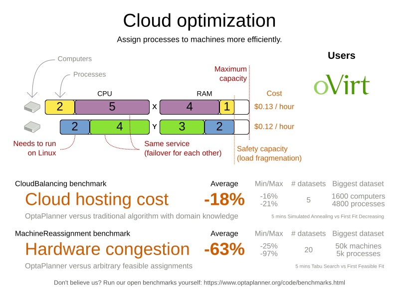
Suppose your company owns a number of cloud computers and needs to run a number of processes on those computers. Assign each process to a computer.
The following hard constraints must be fulfilled:
-
Every computer must be able to handle the minimum hardware requirements of the sum of its processes:
-
CPU capacity: The CPU power of a computer must be at least the sum of the CPU power required by the processes assigned to that computer.
-
Memory capacity: The RAM memory of a computer must be at least the sum of the RAM memory required by the processes assigned to that computer.
-
Network capacity: The network bandwidth of a computer must be at least the sum of the network bandwidth required by the processes assigned to that computer.
-
The following soft constraints should be optimized:
-
Each computer that has one or more processes assigned, incurs a maintenance cost (which is fixed per computer).
-
Cost: Minimize the total maintenance cost.
-
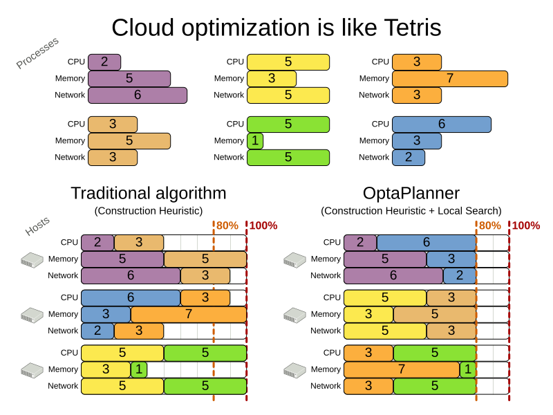
This problem is a form of bin packing. The following is a simplified example, in which we assign four processes to two computers with two constraints (CPU and RAM) with a simple algorithm:
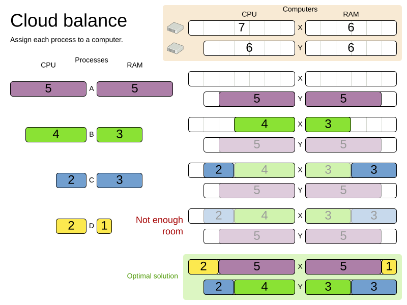
The simple algorithm used here is the First Fit Decreasing algorithm, which assigns the bigger processes first and assigns the smaller processes to the remaining space.
As you can see, it is not optimal, as it does not leave enough room to assign the yellow process D.
OptaPlanner does find the more optimal solution by using additional, smarter algorithms. It also scales: both in data (more processes, more computers) and constraints (more hardware requirements, other constraints). So let’s see how OptaPlanner can be used in this scenario.
Here’s an executive summary of this example and an advanced implementation with more constraints:
3.1.2. Problem size
| Problem Size | Computers | Processes | Search Space |
|---|---|---|---|
2computers-6processes |
2 |
6 |
64 |
3computers-9processes |
3 |
9 |
10^4 |
4computers-12processes |
4 |
12 |
10^7 |
100computers-300processes |
100 |
300 |
10^600 |
200computers-600processes |
200 |
600 |
10^1380 |
400computers-1200processes |
400 |
1200 |
10^3122 |
800computers-2400processes |
800 |
2400 |
10^6967 |
3.2. Using the domain model
3.2.1. Domain model design
Using a domain model helps determine which classes are planning entities and which of their properties are planning variables. It also helps to simplify constraints, improve performance, and increase flexibility for future needs.
To create a domain model, define all the objects that represent the input data for the problem. In this simple example, the objects are processes and computers.
A separate object in the domain model must represent a full data set of problem, which contains the input data as well as a solution. In this example, this object holds a list of computers and a list of processes. Each process is assigned to a computer; the distribution of processes between computers is the solution.
-
Draw a class diagram of your domain model.
-
Normalize it to remove duplicate data.
-
Write down some sample instances for each class.
-
Computer: represents a computer with certain hardware and maintenance costs.In this example, the sample instances for the
Computerclass are:cpuPower,memory,networkBandwidth,cost. -
Process: represents a process with a demand. Needs to be assigned to aComputerby OptaPlanner.Sample instances for
Processare:requiredCpuPower,requiredMemory, andrequiredNetworkBandwidth. -
CloudBalance: represents a problem. Contains everyComputerandProcessfor a certain data set.For an object representing the full data set and solution, a sample instance holding the score must be present. OptaPlanner can calculate and compare the scores for different solutions; the solution with the highest score is the optimal solution. Therefore, the sample instance for
CloudBalanceisscore.
-
-
Determine which relationships (or fields) change during planning.
-
Planning entity: The class (or classes) that OptaPlanner can change during solving. In this example, it is the class
Process, because OptaPlanner can assign processes to computers. -
Problem fact: A class representing input data that OptaPlanner cannot change.
-
Planning variable: The property (or properties) of a planning entity class that changes during solving. In this example, it is the property
computeron the classProcess. -
Planning solution: The class that represents a solution to the problem. This class must represent the full data set and contain all planning entities. In this example that is the class
CloudBalance.
-
In the UML class diagram below, the OptaPlanner concepts are already annotated:
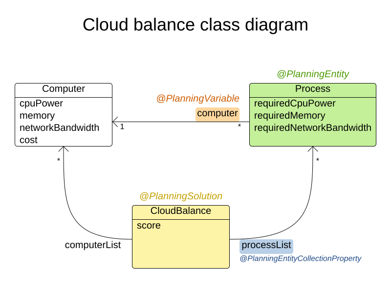
3.2.2. Domain model implementation
The Computer class
The Computer class is a POJO (Plain Old Java Object). Usually, you will have more of this kind of classes with input data.
public class CloudComputer ... {

    private int cpuPower;
    private int memory;
    private int networkBandwidth;
    private int cost;

    ... // getters
}
The Process class
The Process class is particularly important. It is the class that is modified during solving.
We need to tell OptaPlanner that it can change the property computer. To do this:
. Annotate the class with @PlanningEntity.
. Annotate the getter getComputer() with @PlanningVariable.
Of course, the property computer needs a setter too, so OptaPlanner can change it during solving.
@PlanningEntity(...)
public class CloudProcess ... {

    private int requiredCpuPower;
    private int requiredMemory;
    private int requiredNetworkBandwidth;

    private CloudComputer computer;

    ... // getters

    @PlanningVariable
    public CloudComputer getComputer() {
        return computer;
    }

    public void setComputer(CloudComputer computer) {
        computer = computer;
    }

    // ************************************************************************
    // Complex methods
    // ************************************************************************

    ...

}-
OptaPlanner needs to know which values it can choose from to assign to the property
computer. Those values are retrieved from the methodCloudBalance.getComputerList()on the planning solution, which returns a list of all computers in the current data set. -
The
@PlanningVariableautomatically matches with the@ValueRangeProvideronCloudBalance.getComputerList().
|
Instead of getter annotations, it is also possible to use field annotations. |
The CloudBalance class
The CloudBalance class has a @PlanningSolution annotation.
-
It holds a list of all computers and a list of all processes.
-
It represents both the planning problem and (if it is initialized) the planning solution.
-
To save a solution, OptaPlanner initializes a new instance of the class.
-
The
processListproperty holds a list of processes. OptaPlanner can change the processes, allocating them to different computers. Therefore, a process is a planning entity and the list of processes is a collection of planning entities. We annotate the gettergetProcessList()with@PlanningEntityCollectionProperty. -
The
computerListproperty holds a list of computers. OptaPlanner cannot change the computers. Therefore, a computer is a problem fact. Especially for Constraint Streams, the propertycomputerListneeds to be annotated with a@ProblemFactCollectionPropertyso that OptaPlanner can retrieve the list of computers (problem facts) and make it available to the rule engine. -
The
CloudBalanceclass also has a@PlanningScoreannotated propertyscore, which is theScoreof that solution in its current state. OptaPlanner automatically updates it when it calculates aScorefor a solution instance. Therefore, this property needs a setter.
-
@PlanningSolution
public class CloudBalance ... {

    private List<CloudComputer> computerList;

    private List<CloudProcess> processList;

    private HardSoftScore score;

    @ValueRangeProvider
    @ProblemFactCollectionProperty
    public List<CloudComputer> getComputerList() {
        return computerList;
    }

    @PlanningEntityCollectionProperty
    public List<CloudProcess> getProcessList() {
        return processList;
    }

    @PlanningScore
    public HardSoftScore getScore() {
        return score;
    }

    public void setScore(HardSoftScore score) {
        this.score = score;
    }

    ...
}
3.3. Run the cloud balancing Hello World
-
Create a run configuration with the following main class:
org.optaplanner.examples.cloudbalancing.app.CloudBalancingHelloWorldBy default, the Cloud Balancing Hello World is configured to run for 120 seconds.
It executes the following code:
public class CloudBalancingHelloWorld {

    public static void main(String[] args) {
        // Build the Solver
        SolverFactory<CloudBalance> solverFactory = SolverFactory.createFromXmlResource(
                "org/optaplanner/examples/cloudbalancing/solver/cloudBalancingSolverConfig.xml");
        Solver<CloudBalance> solver = solverFactory.buildSolver();

        // Load a problem with 400 computers and 1200 processes
        CloudBalance unsolvedCloudBalance = new CloudBalancingGenerator().createCloudBalance(400, 1200);

        // Solve the problem
        CloudBalance solvedCloudBalance = solver.solve(unsolvedCloudBalance);

        // Display the result
        System.out.println("\nSolved cloudBalance with 400 computers and 1200 processes:\n"
                + toDisplayString(solvedCloudBalance));
    }

    ...
}
The code example does the following:
-
Build the
Solverbased on a solver configuration which can come from an XML file as classpath resource:SolverFactory<CloudBalance> solverFactory = SolverFactory.createFromXmlResource( "org/optaplanner/examples/cloudbalancing/solver/cloudBalancingSolverConfig.xml"); Solver<CloudBalance> solver = solverFactory.buildSolver();Or to avoid XML, build it through the programmatic API instead:
        SolverFactory<CloudBalance> solverFactory = SolverFactory.create(new SolverConfig()
                .withSolutionClass(CloudBalance.class)
                .withEntityClasses(CloudProcess.class)
                .withEasyScoreCalculatorClass(CloudBalancingEasyScoreCalculator.class)
                .withTerminationSpentLimit(Duration.ofMinutes(2)));
        Solver<CloudBalance> solver = solverFactory.buildSolver();
The solver configuration is explained in the next section.
-
Load the problem.
CloudBalancingGeneratorgenerates a random problem: replace this with a class that loads a real problem, for example from a database.CloudBalance unsolvedCloudBalance = new CloudBalancingGenerator().createCloudBalance(400, 1200); -
Solve the problem.
CloudBalance solvedCloudBalance = solver.solve(unsolvedCloudBalance); -
Display the result.
        System.out.println("\nSolved cloudBalance with 400 computers and 1200 processes:\n"
                + toDisplayString(solvedCloudBalance));
3.4. Solver configuration
The solver configuration file determines how the solving process works; it is considered a part of the code.
The file is named cloudBalancingSolverConfig.xml.
<?xml version="1.0" encoding="UTF-8"?>
<solver xmlns="https://www.optaplanner.org/xsd/solver" xmlns:xsi="http://www.w3.org/2001/XMLSchema-instance"
    xsi:schemaLocation="https://www.optaplanner.org/xsd/solver https://www.optaplanner.org/xsd/solver/solver.xsd">
  <!-- Domain model configuration -->
  <solutionClass>org.optaplanner.examples.cloudbalancing.domain.CloudBalance</solutionClass>
  <entityClass>org.optaplanner.examples.cloudbalancing.domain.CloudProcess</entityClass>

  <!-- Score configuration -->
  <scoreDirectorFactory>
    <easyScoreCalculatorClass>org.optaplanner.examples.cloudbalancing.optional.score.CloudBalancingEasyScoreCalculator</easyScoreCalculatorClass>
    <!--<constraintProviderClass>org.optaplanner.examples.cloudbalancing.score.CloudBalancingConstraintProvider</constraintProviderClass>-->
  </scoreDirectorFactory>

  <!-- Optimization algorithms configuration -->
  <termination>
    <secondsSpentLimit>30</secondsSpentLimit>
  </termination>
</solver>
This solver configuration consists of three parts:
-
Domain model configuration: What can OptaPlanner change?
We need to make OptaPlanner aware of our domain classes, annotated with
@PlanningEntityand@PlanningSolutionannotations:<solutionClass>org.optaplanner.examples.cloudbalancing.domain.CloudBalance</solutionClass> <entityClass>org.optaplanner.examples.cloudbalancing.domain.CloudProcess</entityClass> -
Score configuration: How should OptaPlanner optimize the planning variables? What is our goal?
Since we have hard and soft constraints, we use a
HardSoftScore. But we need to tell OptaPlanner how to calculate the score, depending on our business requirements. Further down, we will look into two alternatives to calculate the score, such as using an easy Java implementation, or Constraint Streams.<scoreDirectorFactory> <easyScoreCalculatorClass>org.optaplanner.examples.cloudbalancing.optional.score.CloudBalancingEasyScoreCalculator</easyScoreCalculatorClass> <!--<constraintProviderClass>org.optaplanner.examples.cloudbalancing.score.CloudBalancingConstraintProvider</constraintProviderClass>--> </scoreDirectorFactory> -
Optimization algorithms configuration: How should OptaPlanner optimize it?
In this case, we use the default optimization algorithms (because no explicit optimization algorithms are configured) for 30 seconds:
  <termination>
    <secondsSpentLimit>30</secondsSpentLimit>
  </termination>
OptaPlanner should get a good result in seconds (and even in less than 15 milliseconds with real-time planning), but the more time it has, the better the results. Advanced use cases might use different termination criteria than a hard time limit.
The default algorithms already easily surpass human planners and most in-house implementations. Use the Benchmarker to power tweak to get even better results.
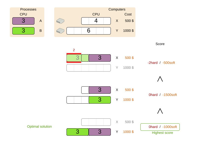
3.5. Score configuration
OptaPlanner searches for the solution with the highest Score.
This example uses a HardSoftScore, which means OptaPlanner looks for the solution with no hard constraints broken (fulfill hardware requirements) and as little as possible soft constraints broken (minimize maintenance cost).
Of course, OptaPlanner needs to be told about these domain-specific score constraints. There are several ways to implement such a score function:
3.5.1. Easy Java score configuration
One way to define a score function is to implement the interface EasyScoreCalculator in plain Java.
  <scoreDirectorFactory>
    <easyScoreCalculatorClass>org.optaplanner.examples.cloudbalancing.optional.score.CloudBalancingEasyScoreCalculator</easyScoreCalculatorClass>
  </scoreDirectorFactory>
Just implement the calculateScore(Solution) method to return a HardSoftScore instance.
public class CloudBalancingEasyScoreCalculator
    implements EasyScoreCalculator<CloudBalance, HardSoftScore> {

    /**
     * A very simple implementation. The double loop can easily be removed by using Maps as shown in
     * {@link CloudBalancingMapBasedEasyScoreCalculator#calculateScore(CloudBalance)}.
     */
    @Override
    public HardSoftScore calculateScore(CloudBalance cloudBalance) {
        int hardScore = 0;
        int softScore = 0;
        for (CloudComputer computer : cloudBalance.getComputerList()) {
            int cpuPowerUsage = 0;
            int memoryUsage = 0;
            int networkBandwidthUsage = 0;
            boolean used = false;

            // Calculate usage
            for (CloudProcess process : cloudBalance.getProcessList()) {
                if (computer.equals(process.getComputer())) {
                    cpuPowerUsage += process.getRequiredCpuPower();
                    memoryUsage += process.getRequiredMemory();
                    networkBandwidthUsage += process.getRequiredNetworkBandwidth();
                    used = true;
                }
            }

            // Hard constraints
            int cpuPowerAvailable = computer.getCpuPower() - cpuPowerUsage;
            if (cpuPowerAvailable < 0) {
                hardScore += cpuPowerAvailable;
            }
            int memoryAvailable = computer.getMemory() - memoryUsage;
            if (memoryAvailable < 0) {
                hardScore += memoryAvailable;
            }
            int networkBandwidthAvailable = computer.getNetworkBandwidth() - networkBandwidthUsage;
            if (networkBandwidthAvailable < 0) {
                hardScore += networkBandwidthAvailable;
            }

            // Soft constraints
            if (used) {
                softScore -= computer.getCost();
            }
        }
        return HardSoftScore.of(hardScore, softScore);
    }

}
Even if we optimize the code above to use Maps to iterate through the processList only once, it is still slow because it does not do incremental score calculation.
To fix that, either use constraint streams, incremental Java score calculation or Drools score calculation.
3.5.2. Constraint streams score configuration
Constraint Streams use incremental calculation.
To use it, implement the interface ConstraintProvider in Java.
  <scoreDirectorFactory>
    <constraintProviderClass>org.optaplanner.examples.cloudbalancing.score.CloudBalancingConstraintProvider</constraintProviderClass>
  </scoreDirectorFactory>
We want to make sure that all computers have enough CPU, RAM and network bandwidth to support all their processes, so we make these hard constraints. If those constraints are met, we want to minimize the maintenance cost, so we add that as a soft constraint.
public class CloudBalancingConstraintProvider implements ConstraintProvider {

    @Override
    public Constraint[] defineConstraints(ConstraintFactory constraintFactory) {
        return new Constraint[] {
                requiredCpuPowerTotal(constraintFactory),
                requiredMemoryTotal(constraintFactory),
                requiredNetworkBandwidthTotal(constraintFactory),
                computerCost(constraintFactory)
        };
    }

    Constraint requiredCpuPowerTotal(ConstraintFactory constraintFactory) {
        return constraintFactory.forEach(CloudProcess.class)
                .groupBy(CloudProcess::getComputer, sum(CloudProcess::getRequiredCpuPower))
                .filter((computer, requiredCpuPower) -> requiredCpuPower > computer.getCpuPower())
                .penalize(HardSoftScore.ONE_HARD,
                        (computer, requiredCpuPower) -> requiredCpuPower - computer.getCpuPower())
                .asConstraint("requiredCpuPowerTotal");
    }

    Constraint requiredMemoryTotal(ConstraintFactory constraintFactory) {
        return constraintFactory.forEach(CloudProcess.class)
                .groupBy(CloudProcess::getComputer, sum(CloudProcess::getRequiredMemory))
                .filter((computer, requiredMemory) -> requiredMemory > computer.getMemory())
                .penalize(HardSoftScore.ONE_HARD,
                        (computer, requiredMemory) -> requiredMemory - computer.getMemory())
                .asConstraint("requiredMemoryTotal");
    }

    Constraint requiredNetworkBandwidthTotal(ConstraintFactory constraintFactory) {
        return constraintFactory.forEach(CloudProcess.class)
                .groupBy(CloudProcess::getComputer, sum(CloudProcess::getRequiredNetworkBandwidth))
                .filter((computer, requiredNetworkBandwidth) -> requiredNetworkBandwidth > computer.getNetworkBandwidth())
                .penalize(HardSoftScore.ONE_HARD,
                        (computer, requiredNetworkBandwidth) -> requiredNetworkBandwidth - computer.getNetworkBandwidth())
                .asConstraint("requiredNetworkBandwidthTotal");
    }

    Constraint computerCost(ConstraintFactory constraintFactory) {
        return constraintFactory.forEach(CloudComputer.class)
                .ifExists(CloudProcess.class, equal(Function.identity(), CloudProcess::getComputer))
                .penalize(HardSoftScore.ONE_SOFT,
                        CloudComputer::getCost)
                .asConstraint("computerCost");
    }

}
3.5.3. Incremental Java score configuration
Another way to define a score function is to implement the interface IncrementalScoreCalculator in plain Java.
  <scoreDirectorFactory>
    <easyScoreCalculatorClass>org.optaplanner.examples.cloudbalancing.optional.score.CloudBalancingIncrementalScoreCalculator</easyScoreCalculatorClass>
</scoreDirectorFactory>public class CloudBalancingIncrementalScoreCalculator
implements IncrementalScoreCalculator<CloudBalance, HardSoftScore> {
private Map<CloudComputer, Integer> cpuPowerUsageMap;
private Map<CloudComputer, Integer> memoryUsageMap;
private Map<CloudComputer, Integer> networkBandwidthUsageMap;
private Map<CloudComputer, Integer> processCountMap;
private int hardScore;
private int softScore;
@Override
public void resetWorkingSolution(CloudBalance cloudBalance) {
int computerListSize = cloudBalance.getComputerList().size();
cpuPowerUsageMap = new HashMap<>(computerListSize);
memoryUsageMap = new HashMap<>(computerListSize);
networkBandwidthUsageMap = new HashMap<>(computerListSize);
processCountMap = new HashMap<>(computerListSize);
for (CloudComputer computer : cloudBalance.getComputerList()) {
cpuPowerUsageMap.put(computer, 0);
memoryUsageMap.put(computer, 0);
networkBandwidthUsageMap.put(computer, 0);
processCountMap.put(computer, 0);
}
hardScore = 0;
softScore = 0;
for (CloudProcess process : cloudBalance.getProcessList()) {
insert(process);
}
}
@Override
public void beforeVariableChanged(Object entity, String variableName) {
retract((CloudProcess) entity);
}
@Override
public void afterVariableChanged(Object entity, String variableName) {
insert((CloudProcess) entity);
}
@Override
public void beforeEntityRemoved(Object entity) {
retract((CloudProcess) entity);
}
...
private void insert(CloudProcess process) {
CloudComputer computer = process.getComputer();
if (computer != null) {
int cpuPower = computer.getCpuPower();
int oldCpuPowerUsage = cpuPowerUsageMap.get(computer);
int oldCpuPowerAvailable = cpuPower - oldCpuPowerUsage;
int newCpuPowerUsage = oldCpuPowerUsage + process.getRequiredCpuPower();
int newCpuPowerAvailable = cpuPower - newCpuPowerUsage;
hardScore += Math.min(newCpuPowerAvailable, 0) - Math.min(oldCpuPowerAvailable, 0);
cpuPowerUsageMap.put(computer, newCpuPowerUsage);
int memory = computer.getMemory();
int oldMemoryUsage = memoryUsageMap.get(computer);
int oldMemoryAvailable = memory - oldMemoryUsage;
int newMemoryUsage = oldMemoryUsage + process.getRequiredMemory();
int newMemoryAvailable = memory - newMemoryUsage;
hardScore += Math.min(newMemoryAvailable, 0) - Math.min(oldMemoryAvailable, 0);
memoryUsageMap.put(computer, newMemoryUsage);
int networkBandwidth = computer.getNetworkBandwidth();
int oldNetworkBandwidthUsage = networkBandwidthUsageMap.get(computer);
int oldNetworkBandwidthAvailable = networkBandwidth - oldNetworkBandwidthUsage;
int newNetworkBandwidthUsage = oldNetworkBandwidthUsage + process.getRequiredNetworkBandwidth();
int newNetworkBandwidthAvailable = networkBandwidth - newNetworkBandwidthUsage;
hardScore += Math.min(newNetworkBandwidthAvailable, 0) - Math.min(oldNetworkBandwidthAvailable, 0);
networkBandwidthUsageMap.put(computer, newNetworkBandwidthUsage);
int oldProcessCount = processCountMap.get(computer);
if (oldProcessCount == 0) {
softScore -= computer.getCost();
}
int newProcessCount = oldProcessCount + 1;
processCountMap.put(computer, newProcessCount);
}
}
private void retract(CloudProcess process) {
CloudComputer computer = process.getComputer();
if (computer != null) {
int cpuPower = computer.getCpuPower();
int oldCpuPowerUsage = cpuPowerUsageMap.get(computer);
int oldCpuPowerAvailable = cpuPower - oldCpuPowerUsage;
int newCpuPowerUsage = oldCpuPowerUsage - process.getRequiredCpuPower();
int newCpuPowerAvailable = cpuPower - newCpuPowerUsage;
hardScore += Math.min(newCpuPowerAvailable, 0) - Math.min(oldCpuPowerAvailable, 0);
cpuPowerUsageMap.put(computer, newCpuPowerUsage);
int memory = computer.getMemory();
int oldMemoryUsage = memoryUsageMap.get(computer);
int oldMemoryAvailable = memory - oldMemoryUsage;
int newMemoryUsage = oldMemoryUsage - process.getRequiredMemory();
int newMemoryAvailable = memory - newMemoryUsage;
hardScore += Math.min(newMemoryAvailable, 0) - Math.min(oldMemoryAvailable, 0);
memoryUsageMap.put(computer, newMemoryUsage);
int networkBandwidth = computer.getNetworkBandwidth();
int oldNetworkBandwidthUsage = networkBandwidthUsageMap.get(computer);
int oldNetworkBandwidthAvailable = networkBandwidth - oldNetworkBandwidthUsage;
int newNetworkBandwidthUsage = oldNetworkBandwidthUsage - process.getRequiredNetworkBandwidth();
int newNetworkBandwidthAvailable = networkBandwidth - newNetworkBandwidthUsage;
hardScore += Math.min(newNetworkBandwidthAvailable, 0) - Math.min(oldNetworkBandwidthAvailable, 0);
networkBandwidthUsageMap.put(computer, newNetworkBandwidthUsage);
int oldProcessCount = processCountMap.get(computer);
int newProcessCount = oldProcessCount - 1;
if (newProcessCount == 0) {
softScore += computer.getCost();
}
processCountMap.put(computer, newProcessCount);
}
}
@Override
public HardSoftScore calculateScore() {
return HardSoftScore.of(hardScore, softScore);
}
}This score calculation is the fastest we can possibly make it. It reacts to every planning variable change, making the smallest possible adjustment to the score.
3.6. Beyond this tutorial
Now that this simple example works, you can try going further. For example, you can enrich the domain model and add extra constraints such as these:
-
Each
Processbelongs to aService. A computer might crash, so processes running the same service must be assigned to different computers. -
Each
Computeris located in aBuilding. A building might burn down, so processes of the same services should (or must) be assigned to computers in different buildings.
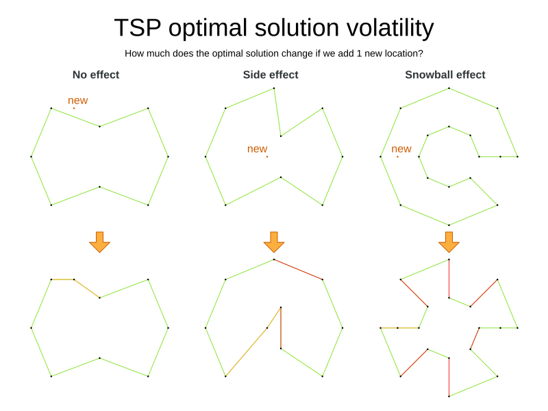
4. Traveling salesman (TSP - traveling salesman problem)
4.1. Problem description
Given a list of cities, find the shortest tour for a salesman that visits each city exactly once.
The problem is defined by Wikipedia. It is one of the most intensively studied problems in computational mathematics. Yet, in the real world, it is often only part of a planning problem, along with other constraints, such as employee shift rostering constraints.
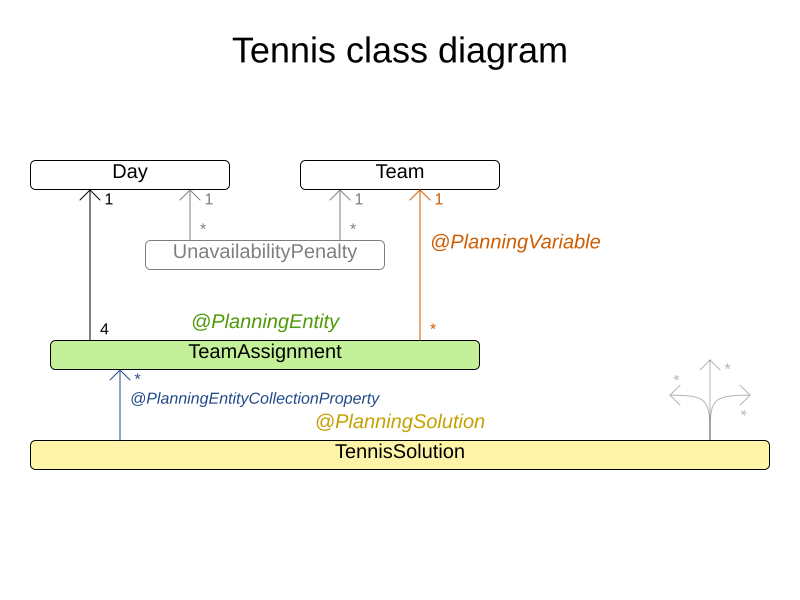
5. Tennis club scheduling
5.1. Problem description
Every week the tennis club has four teams playing round robin against each other. Assign those four spots to the teams fairly.
Hard constraints:
-
Conflict: A team can only play once per day.
-
Unavailability: Some teams are unavailable on some dates.
Medium constraints:
-
Fair assignment: All teams should play an (almost) equal number of times.
Soft constraints:
-
Evenly confrontation: Each team should play against every other team an equal number of times.
6. Meeting scheduling
6.1. Problem description
Assign each meeting to a starting time and a room. Meetings have different durations.
Hard constraints:
-
Room conflict: two meetings must not use the same room at the same time.
-
Required attendance: A person cannot have two required meetings at the same time.
-
Required room capacity: A meeting must not be in a room that doesn’t fit all of the meeting’s attendees.
-
Start and end on same day: A meeting shouldn’t be scheduled over multiple days.
Medium constraints:
-
Preferred attendance: A person cannot have two preferred meetings at the same time, nor a preferred and a required meeting at the same time.
Soft constraints:
-
Sooner rather than later: Schedule all meetings as soon as possible.
-
A break between meetings: Any two meetings should have at least one time grain break between them.
-
Overlapping meetings: To minimize the number of meetings in parallel so people don’t have to choose one meeting over the other.
-
Assign larger rooms first: If a larger room is available any meeting should be assigned to that room in order to accommodate as many people as possible even if they haven’t signed up to that meeting.
-
Room stability: If a person has two consecutive meetings with two or less time grains break between them they better be in the same room.
6.2. Problem size
50meetings-160timegrains-5rooms  has  50 meetings, 160 timeGrains and 5 rooms with a search space of 10^145.
100meetings-320timegrains-5rooms has 100 meetings, 320 timeGrains and 5 rooms with a search space of 10^320.
200meetings-640timegrains-5rooms has 200 meetings, 640 timeGrains and 5 rooms with a search space of 10^701.
400meetings-1280timegrains-5rooms has 400 meetings, 1280 timeGrains and 5 rooms with a search space of 10^1522.
800meetings-2560timegrains-5rooms has 800 meetings, 2560 timeGrains and 5 rooms with a search space of 10^3285.
7. Course timetabling (ITC 2007 Track 3 - Curriculum Course Scheduling)
7.1. Problem description
Schedule each lecture into a timeslot and into a room.
Hard constraints:
-
Teacher conflict: A teacher must not have two lectures in the same period.
-
Curriculum conflict: A curriculum must not have two lectures in the same period.
-
Room occupancy: two lectures must not be in the same room in the same period.
-
Unavailable period (specified per dataset): A specific lecture must not be assigned to a specific period.
Soft constraints:
-
Room capacity: A room’s capacity should not be less than the number of students in its lecture.
-
Minimum working days: Lectures of the same course should be spread out into a minimum number of days.
-
Curriculum compactness: Lectures belonging to the same curriculum should be adjacent to each other (so in consecutive periods).
-
Room stability: Lectures of the same course should be assigned to the same room.
The problem is defined by the International Timetabling Competition 2007 track 3.
7.2. Problem size
comp01 has 24 teachers,  14 curricula,  30 courses, 160 lectures, 30 periods,  6 rooms and   53 unavailable period constraints with a search space of  10^360.
comp02 has 71 teachers,  70 curricula,  82 courses, 283 lectures, 25 periods, 16 rooms and  513 unavailable period constraints with a search space of  10^736.
comp03 has 61 teachers,  68 curricula,  72 courses, 251 lectures, 25 periods, 16 rooms and  382 unavailable period constraints with a search space of  10^653.
comp04 has 70 teachers,  57 curricula,  79 courses, 286 lectures, 25 periods, 18 rooms and  396 unavailable period constraints with a search space of  10^758.
comp05 has 47 teachers, 139 curricula,  54 courses, 152 lectures, 36 periods,  9 rooms and  771 unavailable period constraints with a search space of  10^381.
comp06 has 87 teachers,  70 curricula, 108 courses, 361 lectures, 25 periods, 18 rooms and  632 unavailable period constraints with a search space of  10^957.
comp07 has 99 teachers,  77 curricula, 131 courses, 434 lectures, 25 periods, 20 rooms and  667 unavailable period constraints with a search space of 10^1171.
comp08 has 76 teachers,  61 curricula,  86 courses, 324 lectures, 25 periods, 18 rooms and  478 unavailable period constraints with a search space of  10^859.
comp09 has 68 teachers,  75 curricula,  76 courses, 279 lectures, 25 periods, 18 rooms and  405 unavailable period constraints with a search space of  10^740.
comp10 has 88 teachers,  67 curricula, 115 courses, 370 lectures, 25 periods, 18 rooms and  694 unavailable period constraints with a search space of  10^981.
comp11 has 24 teachers,  13 curricula,  30 courses, 162 lectures, 45 periods,  5 rooms and   94 unavailable period constraints with a search space of  10^381.
comp12 has 74 teachers, 150 curricula,  88 courses, 218 lectures, 36 periods, 11 rooms and 1368 unavailable period constraints with a search space of  10^566.
comp13 has 77 teachers,  66 curricula,  82 courses, 308 lectures, 25 periods, 19 rooms and  468 unavailable period constraints with a search space of  10^824.
comp14 has 68 teachers,  60 curricula,  85 courses, 275 lectures, 25 periods, 17 rooms and  486 unavailable period constraints with a search space of  10^722.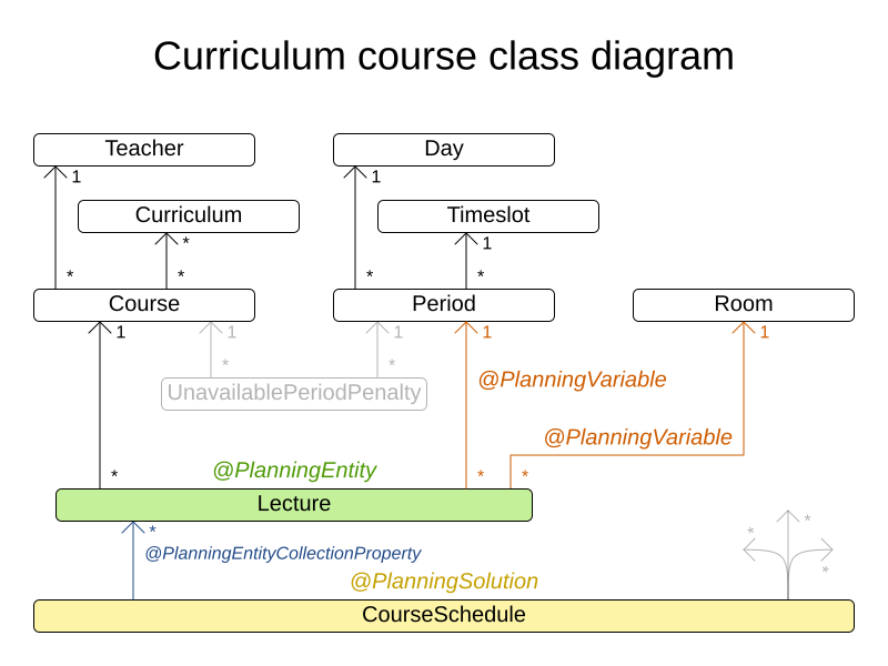
8. Machine reassignment (Google ROADEF 2012)
8.1. Problem description
Assign each process to a machine. All processes already have an original (unoptimized) assignment. Each process requires an amount of each resource (such as CPU, RAM, …). This is a more complex version of the Cloud Balancing example.
Hard constraints:
-
Maximum capacity: The maximum capacity for each resource for each machine must not be exceeded.
-
Conflict: Processes of the same service must run on distinct machines.
-
Spread: Processes of the same service must be spread out across locations.
-
Dependency: The processes of a service depending on another service must run in the neighborhood of a process of the other service.
-
Transient usage: Some resources are transient and count towards the maximum capacity of both the original machine as the newly assigned machine.
Soft constraints:
-
Load: The safety capacity for each resource for each machine should not be exceeded.
-
Balance: Leave room for future assignments by balancing the available resources on each machine.
-
Process move cost: A process has a move cost.
-
Service move cost: A service has a move cost.
-
Machine move cost: Moving a process from machine A to machine B has another A-B specific move cost.
The problem is defined by the Google ROADEF/EURO Challenge 2012.
8.3. Problem size
model_a1_1 has  2 resources,  1 neighborhoods,   4 locations,    4 machines,    79 services,   100 processes and 1 balancePenalties with a search space of     10^60.
model_a1_2 has  4 resources,  2 neighborhoods,   4 locations,  100 machines,   980 services,  1000 processes and 0 balancePenalties with a search space of   10^2000.
model_a1_3 has  3 resources,  5 neighborhoods,  25 locations,  100 machines,   216 services,  1000 processes and 0 balancePenalties with a search space of   10^2000.
model_a1_4 has  3 resources, 50 neighborhoods,  50 locations,   50 machines,   142 services,  1000 processes and 1 balancePenalties with a search space of   10^1698.
model_a1_5 has  4 resources,  2 neighborhoods,   4 locations,   12 machines,   981 services,  1000 processes and 1 balancePenalties with a search space of   10^1079.
model_a2_1 has  3 resources,  1 neighborhoods,   1 locations,  100 machines,  1000 services,  1000 processes and 0 balancePenalties with a search space of   10^2000.
model_a2_2 has 12 resources,  5 neighborhoods,  25 locations,  100 machines,   170 services,  1000 processes and 0 balancePenalties with a search space of   10^2000.
model_a2_3 has 12 resources,  5 neighborhoods,  25 locations,  100 machines,   129 services,  1000 processes and 0 balancePenalties with a search space of   10^2000.
model_a2_4 has 12 resources,  5 neighborhoods,  25 locations,   50 machines,   180 services,  1000 processes and 1 balancePenalties with a search space of   10^1698.
model_a2_5 has 12 resources,  5 neighborhoods,  25 locations,   50 machines,   153 services,  1000 processes and 0 balancePenalties with a search space of   10^1698.
model_b_1  has 12 resources,  5 neighborhoods,  10 locations,  100 machines,  2512 services,  5000 processes and 0 balancePenalties with a search space of  10^10000.
model_b_2  has 12 resources,  5 neighborhoods,  10 locations,  100 machines,  2462 services,  5000 processes and 1 balancePenalties with a search space of  10^10000.
model_b_3  has  6 resources,  5 neighborhoods,  10 locations,  100 machines, 15025 services, 20000 processes and 0 balancePenalties with a search space of  10^40000.
model_b_4  has  6 resources,  5 neighborhoods,  50 locations,  500 machines,  1732 services, 20000 processes and 1 balancePenalties with a search space of  10^53979.
model_b_5  has  6 resources,  5 neighborhoods,  10 locations,  100 machines, 35082 services, 40000 processes and 0 balancePenalties with a search space of  10^80000.
model_b_6  has  6 resources,  5 neighborhoods,  50 locations,  200 machines, 14680 services, 40000 processes and 1 balancePenalties with a search space of  10^92041.
model_b_7  has  6 resources,  5 neighborhoods,  50 locations, 4000 machines, 15050 services, 40000 processes and 1 balancePenalties with a search space of 10^144082.
model_b_8  has  3 resources,  5 neighborhoods,  10 locations,  100 machines, 45030 services, 50000 processes and 0 balancePenalties with a search space of 10^100000.
model_b_9  has  3 resources,  5 neighborhoods, 100 locations, 1000 machines,  4609 services, 50000 processes and 1 balancePenalties with a search space of 10^150000.
model_b_10 has  3 resources,  5 neighborhoods, 100 locations, 5000 machines,  4896 services, 50000 processes and 1 balancePenalties with a search space of 10^184948.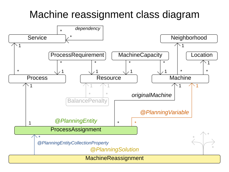
9. Vehicle routing
9.1. Problem description
Using a fleet of vehicles, pick up the objects of each customer and bring them to the depot. Each vehicle can service multiple customers, but it has a limited capacity.
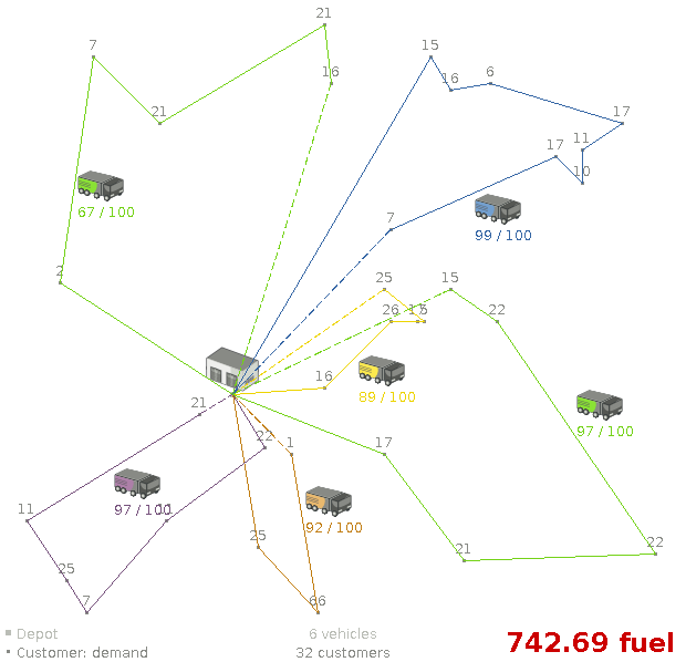
Besides the basic case (CVRP), there is also a variant with time windows (CVRPTW).
Hard constraints:
-
Vehicle capacity: a vehicle cannot carry more items then its capacity.
-
Time windows (only in CVRPTW):
-
Travel time: Traveling from one location to another takes time.
-
Customer service duration: a vehicle must stay at the customer for the length of the service duration.
-
Customer ready time: a vehicle may arrive before the customer’s ready time, but it must wait until the ready time before servicing.
-
Customer due time: a vehicle must arrive on time, before the customer’s due time.
-
Soft constraints:
-
Total distance: minimize the total distance driven (fuel consumption) of all vehicles.
The capacitated vehicle routing problem (CVRP) and its timewindowed variant (CVRPTW) are defined by the VRP web.
9.3. Problem size
CVRP instances (without time windows):
belgium-n50-k10             has  1 depots, 10 vehicles and   49 customers with a search space of   10^74.
belgium-n100-k10            has  1 depots, 10 vehicles and   99 customers with a search space of  10^170.
belgium-n500-k20            has  1 depots, 20 vehicles and  499 customers with a search space of 10^1168.
belgium-n1000-k20           has  1 depots, 20 vehicles and  999 customers with a search space of 10^2607.
belgium-n2750-k55           has  1 depots, 55 vehicles and 2749 customers with a search space of 10^8380.
belgium-road-km-n50-k10     has  1 depots, 10 vehicles and   49 customers with a search space of   10^74.
belgium-road-km-n100-k10    has  1 depots, 10 vehicles and   99 customers with a search space of  10^170.
belgium-road-km-n500-k20    has  1 depots, 20 vehicles and  499 customers with a search space of 10^1168.
belgium-road-km-n1000-k20   has  1 depots, 20 vehicles and  999 customers with a search space of 10^2607.
belgium-road-km-n2750-k55   has  1 depots, 55 vehicles and 2749 customers with a search space of 10^8380.
belgium-road-time-n50-k10   has  1 depots, 10 vehicles and   49 customers with a search space of   10^74.
belgium-road-time-n100-k10  has  1 depots, 10 vehicles and   99 customers with a search space of  10^170.
belgium-road-time-n500-k20  has  1 depots, 20 vehicles and  499 customers with a search space of 10^1168.
belgium-road-time-n1000-k20 has  1 depots, 20 vehicles and  999 customers with a search space of 10^2607.
belgium-road-time-n2750-k55 has  1 depots, 55 vehicles and 2749 customers with a search space of 10^8380.
belgium-d2-n50-k10          has  2 depots, 10 vehicles and   48 customers with a search space of   10^74.
belgium-d3-n100-k10         has  3 depots, 10 vehicles and   97 customers with a search space of  10^170.
belgium-d5-n500-k20         has  5 depots, 20 vehicles and  495 customers with a search space of 10^1168.
belgium-d8-n1000-k20        has  8 depots, 20 vehicles and  992 customers with a search space of 10^2607.
belgium-d10-n2750-k55       has 10 depots, 55 vehicles and 2740 customers with a search space of 10^8380.

A-n32-k5  has 1 depots,  5 vehicles and  31 customers with a search space of  10^40.
A-n33-k5  has 1 depots,  5 vehicles and  32 customers with a search space of  10^41.
A-n33-k6  has 1 depots,  6 vehicles and  32 customers with a search space of  10^42.
A-n34-k5  has 1 depots,  5 vehicles and  33 customers with a search space of  10^43.
A-n36-k5  has 1 depots,  5 vehicles and  35 customers with a search space of  10^46.
A-n37-k5  has 1 depots,  5 vehicles and  36 customers with a search space of  10^48.
A-n37-k6  has 1 depots,  6 vehicles and  36 customers with a search space of  10^49.
A-n38-k5  has 1 depots,  5 vehicles and  37 customers with a search space of  10^49.
A-n39-k5  has 1 depots,  5 vehicles and  38 customers with a search space of  10^51.
A-n39-k6  has 1 depots,  6 vehicles and  38 customers with a search space of  10^52.
A-n44-k7  has 1 depots,  7 vehicles and  43 customers with a search space of  10^61.
A-n45-k6  has 1 depots,  6 vehicles and  44 customers with a search space of  10^62.
A-n45-k7  has 1 depots,  7 vehicles and  44 customers with a search space of  10^63.
A-n46-k7  has 1 depots,  7 vehicles and  45 customers with a search space of  10^65.
A-n48-k7  has 1 depots,  7 vehicles and  47 customers with a search space of  10^68.
A-n53-k7  has 1 depots,  7 vehicles and  52 customers with a search space of  10^77.
A-n54-k7  has 1 depots,  7 vehicles and  53 customers with a search space of  10^79.
A-n55-k9  has 1 depots,  9 vehicles and  54 customers with a search space of  10^82.
A-n60-k9  has 1 depots,  9 vehicles and  59 customers with a search space of  10^91.
A-n61-k9  has 1 depots,  9 vehicles and  60 customers with a search space of  10^93.
A-n62-k8  has 1 depots,  8 vehicles and  61 customers with a search space of  10^94.
A-n63-k9  has 1 depots,  9 vehicles and  62 customers with a search space of  10^97.
A-n63-k10 has 1 depots, 10 vehicles and  62 customers with a search space of  10^98.
A-n64-k9  has 1 depots,  9 vehicles and  63 customers with a search space of  10^99.
A-n65-k9  has 1 depots,  9 vehicles and  64 customers with a search space of 10^101.
A-n69-k9  has 1 depots,  9 vehicles and  68 customers with a search space of 10^108.
A-n80-k10 has 1 depots, 10 vehicles and  79 customers with a search space of 10^130.
F-n45-k4  has 1 depots,  4 vehicles and  44 customers with a search space of  10^60.
F-n72-k4  has 1 depots,  4 vehicles and  71 customers with a search space of 10^108.
F-n135-k7 has 1 depots,  7 vehicles and 134 customers with a search space of 10^240.
CVRPTW instances (with time windows):
belgium-tw-d2-n50-k10    has  2 depots, 10 vehicles and   48 customers with a search space of   10^74.
belgium-tw-d3-n100-k10   has  3 depots, 10 vehicles and   97 customers with a search space of  10^170.
belgium-tw-d5-n500-k20   has  5 depots, 20 vehicles and  495 customers with a search space of 10^1168.
belgium-tw-d8-n1000-k20  has  8 depots, 20 vehicles and  992 customers with a search space of 10^2607.
belgium-tw-d10-n2750-k55 has 10 depots, 55 vehicles and 2740 customers with a search space of 10^8380.
belgium-tw-n50-k10       has  1 depots, 10 vehicles and   49 customers with a search space of   10^74.
belgium-tw-n100-k10      has  1 depots, 10 vehicles and   99 customers with a search space of  10^170.
belgium-tw-n500-k20      has  1 depots, 20 vehicles and  499 customers with a search space of 10^1168.
belgium-tw-n1000-k20     has  1 depots, 20 vehicles and  999 customers with a search space of 10^2607.
belgium-tw-n2750-k55     has  1 depots, 55 vehicles and 2749 customers with a search space of 10^8380.

Solomon_025_C101       has 1 depots,  25 vehicles and   25 customers with a search space of   10^40.
Solomon_025_C201       has 1 depots,  25 vehicles and   25 customers with a search space of   10^40.
Solomon_025_R101       has 1 depots,  25 vehicles and   25 customers with a search space of   10^40.
Solomon_025_R201       has 1 depots,  25 vehicles and   25 customers with a search space of   10^40.
Solomon_025_RC101      has 1 depots,  25 vehicles and   25 customers with a search space of   10^40.
Solomon_025_RC201      has 1 depots,  25 vehicles and   25 customers with a search space of   10^40.
Solomon_100_C101       has 1 depots,  25 vehicles and  100 customers with a search space of  10^185.
Solomon_100_C201       has 1 depots,  25 vehicles and  100 customers with a search space of  10^185.
Solomon_100_R101       has 1 depots,  25 vehicles and  100 customers with a search space of  10^185.
Solomon_100_R201       has 1 depots,  25 vehicles and  100 customers with a search space of  10^185.
Solomon_100_RC101      has 1 depots,  25 vehicles and  100 customers with a search space of  10^185.
Solomon_100_RC201      has 1 depots,  25 vehicles and  100 customers with a search space of  10^185.
Homberger_0200_C1_2_1  has 1 depots,  50 vehicles and  200 customers with a search space of  10^429.
Homberger_0200_C2_2_1  has 1 depots,  50 vehicles and  200 customers with a search space of  10^429.
Homberger_0200_R1_2_1  has 1 depots,  50 vehicles and  200 customers with a search space of  10^429.
Homberger_0200_R2_2_1  has 1 depots,  50 vehicles and  200 customers with a search space of  10^429.
Homberger_0200_RC1_2_1 has 1 depots,  50 vehicles and  200 customers with a search space of  10^429.
Homberger_0200_RC2_2_1 has 1 depots,  50 vehicles and  200 customers with a search space of  10^429.
Homberger_0400_C1_4_1  has 1 depots, 100 vehicles and  400 customers with a search space of  10^978.
Homberger_0400_C2_4_1  has 1 depots, 100 vehicles and  400 customers with a search space of  10^978.
Homberger_0400_R1_4_1  has 1 depots, 100 vehicles and  400 customers with a search space of  10^978.
Homberger_0400_R2_4_1  has 1 depots, 100 vehicles and  400 customers with a search space of  10^978.
Homberger_0400_RC1_4_1 has 1 depots, 100 vehicles and  400 customers with a search space of  10^978.
Homberger_0400_RC2_4_1 has 1 depots, 100 vehicles and  400 customers with a search space of  10^978.
Homberger_0600_C1_6_1  has 1 depots, 150 vehicles and  600 customers with a search space of 10^1571.
Homberger_0600_C2_6_1  has 1 depots, 150 vehicles and  600 customers with a search space of 10^1571.
Homberger_0600_R1_6_1  has 1 depots, 150 vehicles and  600 customers with a search space of 10^1571.
Homberger_0600_R2_6_1  has 1 depots, 150 vehicles and  600 customers with a search space of 10^1571.
Homberger_0600_RC1_6_1 has 1 depots, 150 vehicles and  600 customers with a search space of 10^1571.
Homberger_0600_RC2_6_1 has 1 depots, 150 vehicles and  600 customers with a search space of 10^1571.
Homberger_0800_C1_8_1  has 1 depots, 200 vehicles and  800 customers with a search space of 10^2195.
Homberger_0800_C2_8_1  has 1 depots, 200 vehicles and  800 customers with a search space of 10^2195.
Homberger_0800_R1_8_1  has 1 depots, 200 vehicles and  800 customers with a search space of 10^2195.
Homberger_0800_R2_8_1  has 1 depots, 200 vehicles and  800 customers with a search space of 10^2195.
Homberger_0800_RC1_8_1 has 1 depots, 200 vehicles and  800 customers with a search space of 10^2195.
Homberger_0800_RC2_8_1 has 1 depots, 200 vehicles and  800 customers with a search space of 10^2195.
Homberger_1000_C110_1  has 1 depots, 250 vehicles and 1000 customers with a search space of 10^2840.
Homberger_1000_C210_1  has 1 depots, 250 vehicles and 1000 customers with a search space of 10^2840.
Homberger_1000_R110_1  has 1 depots, 250 vehicles and 1000 customers with a search space of 10^2840.
Homberger_1000_R210_1  has 1 depots, 250 vehicles and 1000 customers with a search space of 10^2840.
Homberger_1000_RC110_1 has 1 depots, 250 vehicles and 1000 customers with a search space of 10^2840.
Homberger_1000_RC210_1 has 1 depots, 250 vehicles and 1000 customers with a search space of 10^2840.
9.4. Domain model
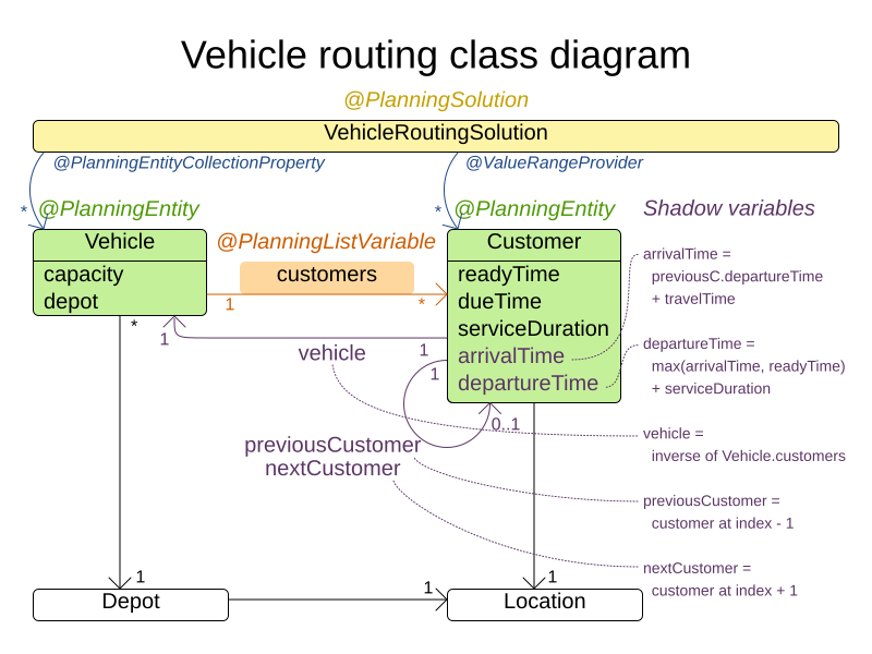
The vehicle routing with timewindows domain model makes heavily use of shadow variables.
This allows it to express its constraints more naturally, because properties such as arrivalTime and departureTime, are directly available on the domain model.
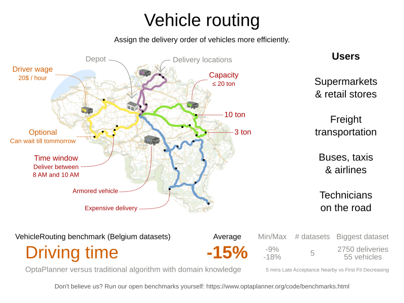
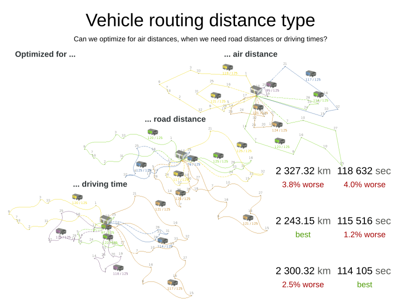
9.4.1. Road distances instead of air distances
In the real world, vehicles cannot follow a straight line from location to location: they have to use roads and highways. From a business point of view, this matters a lot:
For the optimization algorithm, this does not matter much, as long as the distance between two points can be looked up (and are preferably precalculated). The road cost does not even need to be a distance, it can also be travel time, fuel cost, or a weighted function of those. There are several technologies available to precalculate road costs, such as GraphHopper (embeddable, offline Java engine), Open MapQuest (web service) and Google Maps Client API (web service).
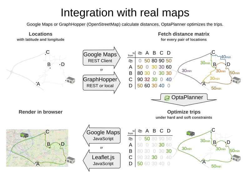
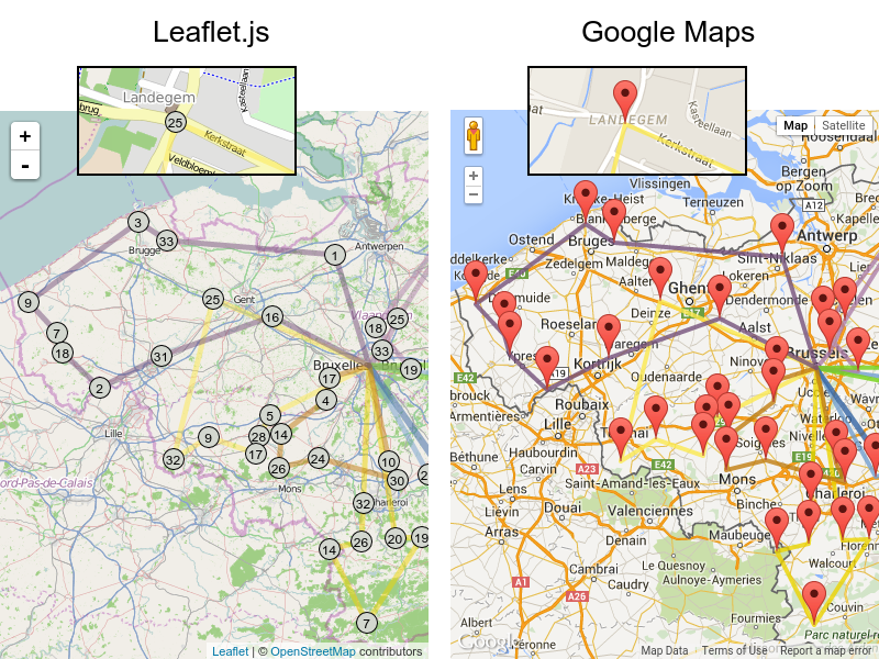
There are also several technologies to render it, such as Leaflet and Google Maps for developers:
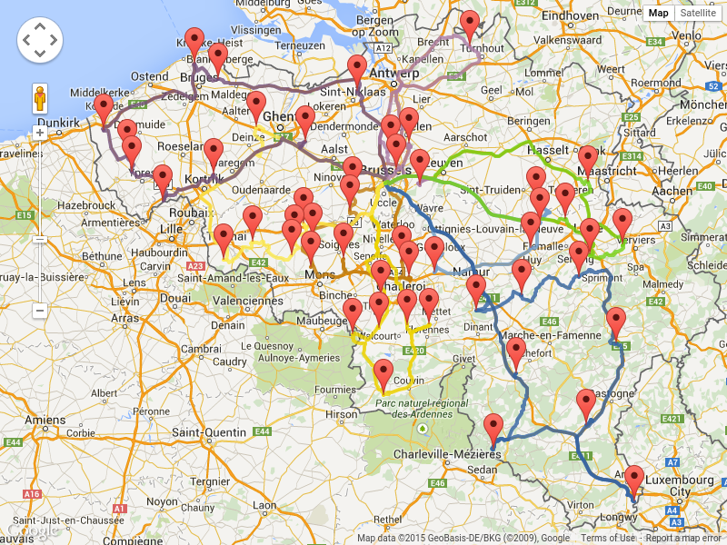
It is even possible to render the actual road routes with GraphHopper or Google Map Directions, but because of route overlaps on highways, it can become harder to see the standstill order:
Take special care that the road costs between two points use the same optimization criteria as the one used in OptaPlanner. For example, GraphHopper etc will by default return the fastest route, not the shortest route. Don’t use the km (or miles) distances of the fastest GPS routes to optimize the shortest trip in OptaPlanner: this leads to a suboptimal solution as shown below:
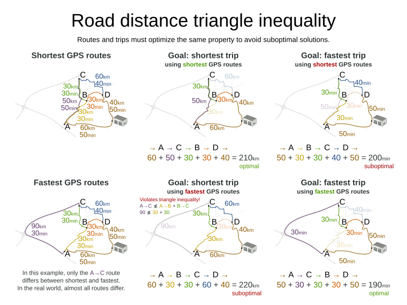
Contrary to popular belief, most users do not want the shortest route: they want the fastest route instead. They prefer highways over normal roads. They prefer normal roads over dirt roads. In the real world, the fastest and shortest route are rarely the same.
10. Project job scheduling
10.1. Problem description
Schedule all jobs in time and execution mode to minimize project delays. Each job is part of a project. A job can be executed in different ways: each way is an execution mode that implies a different duration but also different resource usages. This is a form of flexible job shop scheduling.
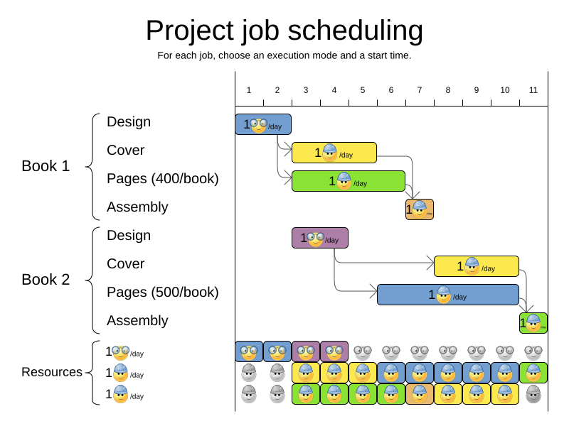
Hard constraints:
-
Job precedence: a job can only start when all its predecessor jobs are finished.
-
Resource capacity: do not use more resources than available.
-
Resources are local (shared between jobs of the same project) or global (shared between all jobs)
-
Resources are renewable (capacity available per day) or nonrenewable (capacity available for all days)
-
Medium constraints:
-
Total project delay: minimize the duration (makespan) of each project.
Soft constraints:
-
Total makespan: minimize the duration of the whole multi-project schedule.
The problem is defined by the MISTA 2013 challenge.
10.2. Problem size
Schedule A-1 has 2 projects, 24 jobs, 64 execution modes, 7 resources and 150 resource requirements.
Schedule A-2 has 2 projects, 44 jobs, 124 execution modes, 7 resources and 420 resource requirements.
Schedule A-3 has 2 projects, 64 jobs, 184 execution modes, 7 resources and 630 resource requirements.
Schedule A-4 has 5 projects, 60 jobs, 160 execution modes, 16 resources and 390 resource requirements.
Schedule A-5 has 5 projects, 110 jobs, 310 execution modes, 16 resources and 900 resource requirements.
Schedule A-6 has 5 projects, 160 jobs, 460 execution modes, 16 resources and 1440 resource requirements.
Schedule A-7 has 10 projects, 120 jobs, 320 execution modes, 22 resources and 900 resource requirements.
Schedule A-8 has 10 projects, 220 jobs, 620 execution modes, 22 resources and 1860 resource requirements.
Schedule A-9 has 10 projects, 320 jobs, 920 execution modes, 31 resources and 2880 resource requirements.
Schedule A-10 has 10 projects, 320 jobs, 920 execution modes, 31 resources and 2970 resource requirements.
Schedule B-1 has 10 projects, 120 jobs, 320 execution modes, 31 resources and 900 resource requirements.
Schedule B-2 has 10 projects, 220 jobs, 620 execution modes, 22 resources and 1740 resource requirements.
Schedule B-3 has 10 projects, 320 jobs, 920 execution modes, 31 resources and 3060 resource requirements.
Schedule B-4 has 15 projects, 180 jobs, 480 execution modes, 46 resources and 1530 resource requirements.
Schedule B-5 has 15 projects, 330 jobs, 930 execution modes, 46 resources and 2760 resource requirements.
Schedule B-6 has 15 projects, 480 jobs, 1380 execution modes, 46 resources and 4500 resource requirements.
Schedule B-7 has 20 projects, 240 jobs, 640 execution modes, 61 resources and 1710 resource requirements.
Schedule B-8 has 20 projects, 440 jobs, 1240 execution modes, 42 resources and 3180 resource requirements.
Schedule B-9 has 20 projects, 640 jobs, 1840 execution modes, 61 resources and 5940 resource requirements.
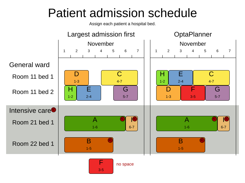
Schedule B-10 has 20 projects, 460 jobs, 1300 execution modes, 42 resources and 4260 resource requirements.11. Hospital bed planning (PAS - Patient Admission Scheduling)
11.1. Problem description
Assign each patient (that will come to the hospital) into a bed for each night that the patient will stay in the hospital. Each bed belongs to a room and each room belongs to a department. The arrival and departure dates of the patients is fixed: only a bed needs to be assigned for each night.
This problem features overconstrained datasets.
Hard constraints:
-
Two patients must not be assigned to the same bed in the same night. Weight:
-1000hard * conflictNightCount. -
A room can have a gender limitation: only females, only males, the same gender in the same night or no gender limitation at all. Weight:
-50hard * nightCount. -
A department can have a minimum or maximum age. Weight:
-100hard * nightCount. -
A patient can require a room with specific equipment(s). Weight:
-50hard * nightCount.
Medium constraints:
-
Assign every patient to a bed, unless the dataset is overconstrained. Weight:
-1medium * nightCount.
Soft constraints:
-
A patient can prefer a maximum room size, for example if he/she wants a single room. Weight:
-8soft * nightCount. -
A patient is best assigned to a department that specializes in his/her problem. Weight:
-10soft * nightCount. -
A patient is best assigned to a room that specializes in his/her problem. Weight:
-20soft * nightCount.-
That room speciality should be priority 1. Weight:
-10soft * (priority - 1) * nightCount.
-
-
A patient can prefer a room with specific equipment(s). Weight:
-20soft * nightCount.
The problem is a variant on Kaho’s Patient Scheduling and the datasets come from real world hospitals.
11.2. Problem size
overconstrained01 has 6 specialisms, 4 equipments, 1 departments,  25 rooms,  69 beds, 14 nights,  519 patients and  519 admissions with a search space of 10^958.
testdata01        has 4 specialisms, 2 equipments, 4 departments,  98 rooms, 286 beds, 14 nights,  652 patients and  652 admissions with a search space of 10^1603.
testdata02        has 6 specialisms, 2 equipments, 6 departments, 151 rooms, 465 beds, 14 nights,  755 patients and  755 admissions with a search space of 10^2015.
testdata03        has 5 specialisms, 2 equipments, 5 departments, 131 rooms, 395 beds, 14 nights,  708 patients and  708 admissions with a search space of 10^1840.
testdata04        has 6 specialisms, 2 equipments, 6 departments, 155 rooms, 471 beds, 14 nights,  746 patients and  746 admissions with a search space of 10^1995.
testdata05        has 4 specialisms, 2 equipments, 4 departments, 102 rooms, 325 beds, 14 nights,  587 patients and  587 admissions with a search space of 10^1476.
testdata06        has 4 specialisms, 2 equipments, 4 departments, 104 rooms, 313 beds, 14 nights,  685 patients and  685 admissions with a search space of 10^1711.
testdata07        has 6 specialisms, 4 equipments, 6 departments, 162 rooms, 472 beds, 14 nights,  519 patients and  519 admissions with a search space of 10^1389.
testdata08        has 6 specialisms, 4 equipments, 6 departments, 148 rooms, 441 beds, 21 nights,  895 patients and  895 admissions with a search space of 10^2368.
testdata09        has 4 specialisms, 4 equipments, 4 departments, 105 rooms, 310 beds, 28 nights, 1400 patients and 1400 admissions with a search space of 10^3490.
testdata10        has 4 specialisms, 4 equipments, 4 departments, 104 rooms, 308 beds, 56 nights, 1575 patients and 1575 admissions with a search space of 10^3922.
testdata11        has 4 specialisms, 4 equipments, 4 departments, 107 rooms, 318 beds, 91 nights, 2514 patients and 2514 admissions with a search space of 10^6295.
testdata12        has 4 specialisms, 4 equipments, 4 departments, 105 rooms, 310 beds, 84 nights, 2750 patients and 2750 admissions with a search space of 10^6856.
testdata13        has 5 specialisms, 4 equipments, 5 departments, 125 rooms, 368 beds, 28 nights,  907 patients and 1109 admissions with a search space of 10^2847.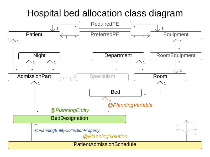
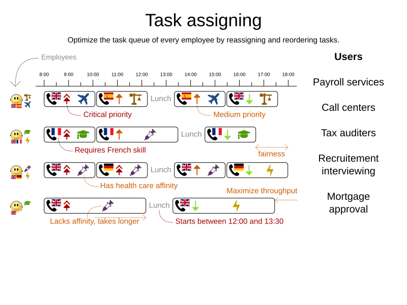
12. Task assigning
12.1. Problem description
Assign each task to a spot in an employee’s queue. Each task has a duration which is affected by the employee’s affinity level with the task’s customer.
Hard constraints:
-
Skill: Each task requires one or more skills. The employee must possess all these skills.
Soft level 0 constraints:
-
Critical tasks: Complete critical tasks first, sooner than major and minor tasks.
Soft level 1 constraints:
-
Minimize makespan: Reduce the time to complete all tasks.
-
Start with the longest working employee first, then the second longest working employee and so forth, to create fairness and load balancing.
-
Soft level 2 constraints:
-
Major tasks: Complete major tasks as soon as possible, sooner than minor tasks.
Soft level 3 constraints:
-
Minor tasks: Complete minor tasks as soon as possible.
12.3. Problem size
24tasks-8employees   has  24 tasks, 6 skills,  8 employees,   4 task types and  4 customers with a search space of   10^30.
50tasks-5employees   has  50 tasks, 5 skills,  5 employees,  10 task types and 10 customers with a search space of   10^69.
100tasks-5employees  has 100 tasks, 5 skills,  5 employees,  20 task types and 15 customers with a search space of  10^164.
500tasks-20employees has 500 tasks, 6 skills, 20 employees, 100 task types and 60 customers with a search space of 10^1168.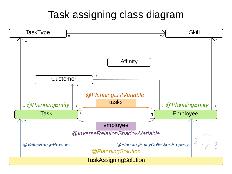
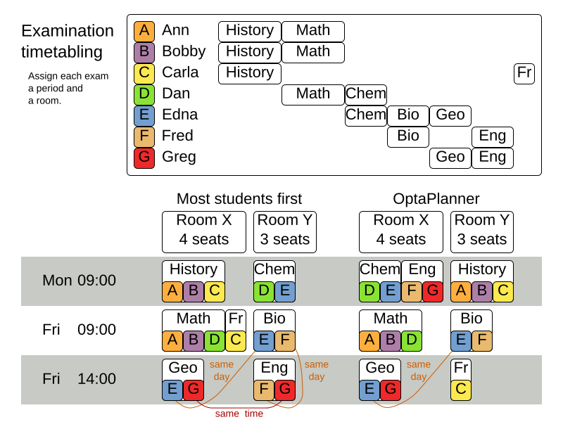
13. Exam timetabling (ITC 2007 track 1 - Examination)
13.1. Problem description
Schedule each exam into a period and into a room. Multiple exams can share the same room during the same period.
Hard constraints:
-
Exam conflict: two exams that share students must not occur in the same period.
-
Room capacity: A room’s seating capacity must suffice at all times.
-
Period duration: A period’s duration must suffice for all of its exams.
-
Period related hard constraints (specified per dataset):
-
Coincidence: two specified exams must use the same period (but possibly another room).
-
Exclusion: two specified exams must not use the same period.
-
After: A specified exam must occur in a period after another specified exam’s period.
-
-
Room related hard constraints (specified per dataset):
-
Exclusive: one specified exam should not have to share its room with any other exam.
-
Soft constraints (each of which has a parametrized penalty):
-
The same student should not have two exams in a row.
-
The same student should not have two exams on the same day.
-
Period spread: two exams that share students should be a number of periods apart.
-
Mixed durations: two exams that share a room should not have different durations.
-
Front load: Large exams should be scheduled earlier in the schedule.
-
Period penalty (specified per dataset): Some periods have a penalty when used.
-
Room penalty (specified per dataset): Some rooms have a penalty when used.
It uses large test data sets of real-life universities.
The problem is defined by the International Timetabling Competition 2007 track 1. Geoffrey De Smet finished 4th in that competition with a very early version of OptaPlanner. Many improvements have been made since then.
13.2. Problem size
exam_comp_set1 has  7883 students,  607 exams, 54 periods,  7 rooms,  12 period constraints and  0 room constraints with a search space of 10^1564.
exam_comp_set2 has 12484 students,  870 exams, 40 periods, 49 rooms,  12 period constraints and  2 room constraints with a search space of 10^2864.
exam_comp_set3 has 16365 students,  934 exams, 36 periods, 48 rooms, 168 period constraints and 15 room constraints with a search space of 10^3023.
exam_comp_set4 has  4421 students,  273 exams, 21 periods,  1 rooms,  40 period constraints and  0 room constraints with a search space of  10^360.
exam_comp_set5 has  8719 students, 1018 exams, 42 periods,  3 rooms,  27 period constraints and  0 room constraints with a search space of 10^2138.
exam_comp_set6 has  7909 students,  242 exams, 16 periods,  8 rooms,  22 period constraints and  0 room constraints with a search space of  10^509.
exam_comp_set7 has 13795 students, 1096 exams, 80 periods, 15 rooms,  28 period constraints and  0 room constraints with a search space of 10^3374.
exam_comp_set8 has  7718 students,  598 exams, 80 periods,  8 rooms,  20 period constraints and  1 room constraints with a search space of 10^1678.
13.3. Domain model
Below you can see the main examination domain classes:
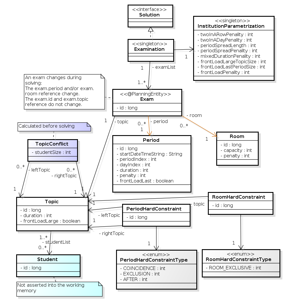
Notice that we’ve split up the exam concept into an Exam class and a Topic class.
The Exam instances change during solving (this is the planning entity class), when their period or room property changes.
The Topic, Period and Room instances never change during solving (these are problem facts, just like some other classes).
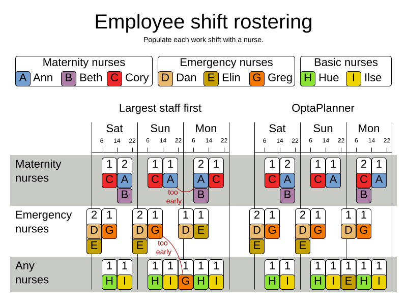
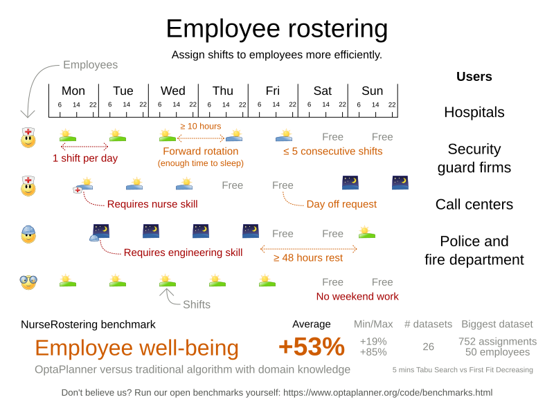
14. Nurse rostering (INRC 2010)
14.1. Problem description
For each shift, assign a nurse to work that shift.
Hard constraints:
-
No unassigned shifts (built-in): Every shift need to be assigned to an employee.
-
Shift conflict: An employee can have only one shift per day.
Soft constraints:
-
Contract obligations. The business frequently violates these, so they decided to define these as soft constraints instead of hard constraints.
-
Minimum and maximum assignments: Each employee needs to work more than x shifts and less than y shifts (depending on their contract).
-
Minimum and maximum consecutive working days: Each employee needs to work between x and y days in a row (depending on their contract).
-
Minimum and maximum consecutive free days: Each employee needs to be free between x and y days in a row (depending on their contract).
-
Minimum and maximum consecutive working weekends: Each employee needs to work between x and y weekends in a row (depending on their contract).
-
Complete weekends: Each employee needs to work every day in a weekend or not at all.
-
Identical shift types during weekend: Each weekend shift for the same weekend of the same employee must be the same shift type.
-
Unwanted patterns: A combination of unwanted shift types in a row. For example: a late shift followed by an early shift followed by a late shift.
-
-
Employee wishes:
-
Day on request: An employee wants to work on a specific day.
-
Day off request: An employee does not want to work on a specific day.
-
Shift on request: An employee wants to be assigned to a specific shift.
-
Shift off request: An employee does not want to be assigned to a specific shift.
-
-
Alternative skill: An employee assigned to a shift should have a proficiency in every skill required by that shift.
The problem is defined by the International Nurse Rostering Competition 2010.
14.3. Problem size
There are three dataset types:
-
sprint: must be solved in seconds.
-
medium: must be solved in minutes.
-
long: must be solved in hours.
toy1          has 1 skills, 3 shiftTypes, 2 patterns, 1 contracts,  6 employees,  7 shiftDates,  35 shiftAssignments and   0 requests with a search space of   10^27.
toy2          has 1 skills, 3 shiftTypes, 3 patterns, 2 contracts, 20 employees, 28 shiftDates, 180 shiftAssignments and 140 requests with a search space of  10^234.

sprint01      has 1 skills, 4 shiftTypes, 3 patterns, 4 contracts, 10 employees, 28 shiftDates, 152 shiftAssignments and 150 requests with a search space of  10^152.
sprint02      has 1 skills, 4 shiftTypes, 3 patterns, 4 contracts, 10 employees, 28 shiftDates, 152 shiftAssignments and 150 requests with a search space of  10^152.
sprint03      has 1 skills, 4 shiftTypes, 3 patterns, 4 contracts, 10 employees, 28 shiftDates, 152 shiftAssignments and 150 requests with a search space of  10^152.
sprint04      has 1 skills, 4 shiftTypes, 3 patterns, 4 contracts, 10 employees, 28 shiftDates, 152 shiftAssignments and 150 requests with a search space of  10^152.
sprint05      has 1 skills, 4 shiftTypes, 3 patterns, 4 contracts, 10 employees, 28 shiftDates, 152 shiftAssignments and 150 requests with a search space of  10^152.
sprint06      has 1 skills, 4 shiftTypes, 3 patterns, 4 contracts, 10 employees, 28 shiftDates, 152 shiftAssignments and 150 requests with a search space of  10^152.
sprint07      has 1 skills, 4 shiftTypes, 3 patterns, 4 contracts, 10 employees, 28 shiftDates, 152 shiftAssignments and 150 requests with a search space of  10^152.
sprint08      has 1 skills, 4 shiftTypes, 3 patterns, 4 contracts, 10 employees, 28 shiftDates, 152 shiftAssignments and 150 requests with a search space of  10^152.
sprint09      has 1 skills, 4 shiftTypes, 3 patterns, 4 contracts, 10 employees, 28 shiftDates, 152 shiftAssignments and 150 requests with a search space of  10^152.
sprint10      has 1 skills, 4 shiftTypes, 3 patterns, 4 contracts, 10 employees, 28 shiftDates, 152 shiftAssignments and 150 requests with a search space of  10^152.
sprint_hint01 has 1 skills, 4 shiftTypes, 8 patterns, 3 contracts, 10 employees, 28 shiftDates, 152 shiftAssignments and 150 requests with a search space of  10^152.
sprint_hint02 has 1 skills, 4 shiftTypes, 0 patterns, 3 contracts, 10 employees, 28 shiftDates, 152 shiftAssignments and 150 requests with a search space of  10^152.
sprint_hint03 has 1 skills, 4 shiftTypes, 8 patterns, 3 contracts, 10 employees, 28 shiftDates, 152 shiftAssignments and 150 requests with a search space of  10^152.
sprint_late01 has 1 skills, 4 shiftTypes, 8 patterns, 3 contracts, 10 employees, 28 shiftDates, 152 shiftAssignments and 150 requests with a search space of  10^152.
sprint_late02 has 1 skills, 3 shiftTypes, 4 patterns, 3 contracts, 10 employees, 28 shiftDates, 144 shiftAssignments and 139 requests with a search space of  10^144.
sprint_late03 has 1 skills, 4 shiftTypes, 8 patterns, 3 contracts, 10 employees, 28 shiftDates, 160 shiftAssignments and 150 requests with a search space of  10^160.
sprint_late04 has 1 skills, 4 shiftTypes, 8 patterns, 3 contracts, 10 employees, 28 shiftDates, 160 shiftAssignments and 150 requests with a search space of  10^160.
sprint_late05 has 1 skills, 4 shiftTypes, 8 patterns, 3 contracts, 10 employees, 28 shiftDates, 152 shiftAssignments and 150 requests with a search space of  10^152.
sprint_late06 has 1 skills, 4 shiftTypes, 0 patterns, 3 contracts, 10 employees, 28 shiftDates, 152 shiftAssignments and 150 requests with a search space of  10^152.
sprint_late07 has 1 skills, 4 shiftTypes, 0 patterns, 3 contracts, 10 employees, 28 shiftDates, 152 shiftAssignments and 150 requests with a search space of  10^152.
sprint_late08 has 1 skills, 4 shiftTypes, 0 patterns, 3 contracts, 10 employees, 28 shiftDates, 152 shiftAssignments and   0 requests with a search space of  10^152.
sprint_late09 has 1 skills, 4 shiftTypes, 0 patterns, 3 contracts, 10 employees, 28 shiftDates, 152 shiftAssignments and   0 requests with a search space of  10^152.
sprint_late10 has 1 skills, 4 shiftTypes, 0 patterns, 3 contracts, 10 employees, 28 shiftDates, 152 shiftAssignments and 150 requests with a search space of  10^152.

medium01      has 1 skills, 4 shiftTypes, 0 patterns, 4 contracts, 31 employees, 28 shiftDates, 608 shiftAssignments and 403 requests with a search space of  10^906.
medium02      has 1 skills, 4 shiftTypes, 0 patterns, 4 contracts, 31 employees, 28 shiftDates, 608 shiftAssignments and 403 requests with a search space of  10^906.
medium03      has 1 skills, 4 shiftTypes, 0 patterns, 4 contracts, 31 employees, 28 shiftDates, 608 shiftAssignments and 403 requests with a search space of  10^906.
medium04      has 1 skills, 4 shiftTypes, 0 patterns, 4 contracts, 31 employees, 28 shiftDates, 608 shiftAssignments and 403 requests with a search space of  10^906.
medium05      has 1 skills, 4 shiftTypes, 0 patterns, 4 contracts, 31 employees, 28 shiftDates, 608 shiftAssignments and 403 requests with a search space of  10^906.
medium_hint01 has 1 skills, 4 shiftTypes, 7 patterns, 4 contracts, 30 employees, 28 shiftDates, 428 shiftAssignments and 390 requests with a search space of  10^632.
medium_hint02 has 1 skills, 4 shiftTypes, 7 patterns, 3 contracts, 30 employees, 28 shiftDates, 428 shiftAssignments and 390 requests with a search space of  10^632.
medium_hint03 has 1 skills, 4 shiftTypes, 7 patterns, 4 contracts, 30 employees, 28 shiftDates, 428 shiftAssignments and 390 requests with a search space of  10^632.
medium_late01 has 1 skills, 4 shiftTypes, 7 patterns, 4 contracts, 30 employees, 28 shiftDates, 424 shiftAssignments and 390 requests with a search space of  10^626.
medium_late02 has 1 skills, 4 shiftTypes, 7 patterns, 3 contracts, 30 employees, 28 shiftDates, 428 shiftAssignments and 390 requests with a search space of  10^632.
medium_late03 has 1 skills, 4 shiftTypes, 0 patterns, 4 contracts, 30 employees, 28 shiftDates, 428 shiftAssignments and 390 requests with a search space of  10^632.
medium_late04 has 1 skills, 4 shiftTypes, 7 patterns, 3 contracts, 30 employees, 28 shiftDates, 416 shiftAssignments and 390 requests with a search space of  10^614.
medium_late05 has 2 skills, 5 shiftTypes, 7 patterns, 4 contracts, 30 employees, 28 shiftDates, 452 shiftAssignments and 390 requests with a search space of  10^667.

long01        has 2 skills, 5 shiftTypes, 3 patterns, 3 contracts, 49 employees, 28 shiftDates, 740 shiftAssignments and 735 requests with a search space of 10^1250.
long02        has 2 skills, 5 shiftTypes, 3 patterns, 3 contracts, 49 employees, 28 shiftDates, 740 shiftAssignments and 735 requests with a search space of 10^1250.
long03        has 2 skills, 5 shiftTypes, 3 patterns, 3 contracts, 49 employees, 28 shiftDates, 740 shiftAssignments and 735 requests with a search space of 10^1250.
long04        has 2 skills, 5 shiftTypes, 3 patterns, 3 contracts, 49 employees, 28 shiftDates, 740 shiftAssignments and 735 requests with a search space of 10^1250.
long05        has 2 skills, 5 shiftTypes, 3 patterns, 3 contracts, 49 employees, 28 shiftDates, 740 shiftAssignments and 735 requests with a search space of 10^1250.
long_hint01   has 2 skills, 5 shiftTypes, 9 patterns, 3 contracts, 50 employees, 28 shiftDates, 740 shiftAssignments and   0 requests with a search space of 10^1257.
long_hint02   has 2 skills, 5 shiftTypes, 7 patterns, 3 contracts, 50 employees, 28 shiftDates, 740 shiftAssignments and   0 requests with a search space of 10^1257.
long_hint03   has 2 skills, 5 shiftTypes, 7 patterns, 3 contracts, 50 employees, 28 shiftDates, 740 shiftAssignments and   0 requests with a search space of 10^1257.
long_late01   has 2 skills, 5 shiftTypes, 9 patterns, 3 contracts, 50 employees, 28 shiftDates, 752 shiftAssignments and   0 requests with a search space of 10^1277.
long_late02   has 2 skills, 5 shiftTypes, 9 patterns, 4 contracts, 50 employees, 28 shiftDates, 752 shiftAssignments and   0 requests with a search space of 10^1277.
long_late03   has 2 skills, 5 shiftTypes, 9 patterns, 3 contracts, 50 employees, 28 shiftDates, 752 shiftAssignments and   0 requests with a search space of 10^1277.
long_late04   has 2 skills, 5 shiftTypes, 9 patterns, 4 contracts, 50 employees, 28 shiftDates, 752 shiftAssignments and   0 requests with a search space of 10^1277.
long_late05   has 2 skills, 5 shiftTypes, 9 patterns, 3 contracts, 50 employees, 28 shiftDates, 740 shiftAssignments and   0 requests with a search space of 10^1257.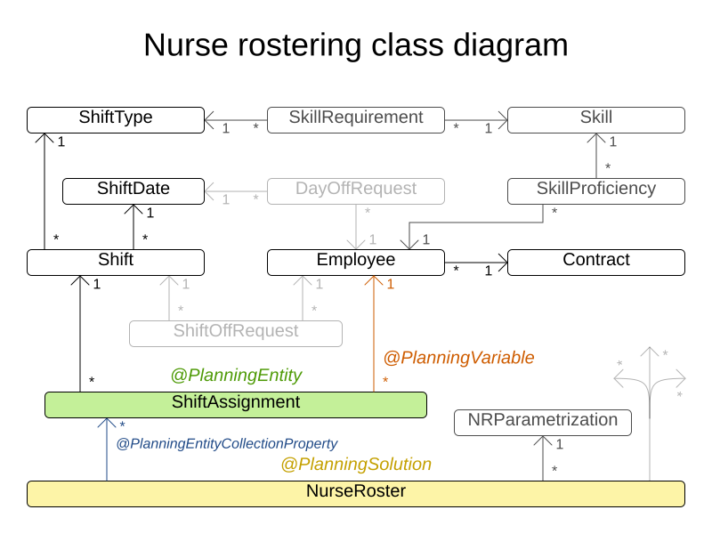
15. Traveling tournament problem (TTP)
15.1. Problem description
Schedule matches between n teams.
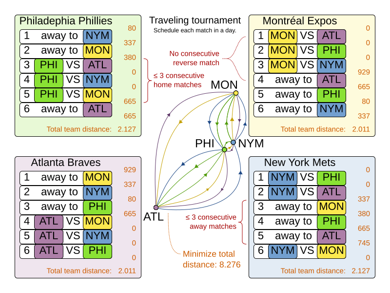
Hard constraints:
-
Each team plays twice against every other team: once home and once away.
-
Each team has exactly one match on each timeslot.
-
No team must have more than three consecutive home or three consecutive away matches.
-
No repeaters: no two consecutive matches of the same two opposing teams.
Soft constraints:
-
Minimize the total distance traveled by all teams.
The problem is defined on Michael Trick’s website (which contains the world records too).
15.2. Problem size
1-nl04     has  6 days,  4 teams and   12 matches with a search space of    10^5.
1-nl06     has 10 days,  6 teams and   30 matches with a search space of   10^19.
1-nl08     has 14 days,  8 teams and   56 matches with a search space of   10^43.
1-nl10     has 18 days, 10 teams and   90 matches with a search space of   10^79.
1-nl12     has 22 days, 12 teams and  132 matches with a search space of  10^126.
1-nl14     has 26 days, 14 teams and  182 matches with a search space of  10^186.
1-nl16     has 30 days, 16 teams and  240 matches with a search space of  10^259.
2-bra24    has 46 days, 24 teams and  552 matches with a search space of  10^692.
3-nfl16    has 30 days, 16 teams and  240 matches with a search space of  10^259.
3-nfl18    has 34 days, 18 teams and  306 matches with a search space of  10^346.
3-nfl20    has 38 days, 20 teams and  380 matches with a search space of  10^447.
3-nfl22    has 42 days, 22 teams and  462 matches with a search space of  10^562.
3-nfl24    has 46 days, 24 teams and  552 matches with a search space of  10^692.
3-nfl26    has 50 days, 26 teams and  650 matches with a search space of  10^838.
3-nfl28    has 54 days, 28 teams and  756 matches with a search space of  10^999.
3-nfl30    has 58 days, 30 teams and  870 matches with a search space of 10^1175.
3-nfl32    has 62 days, 32 teams and  992 matches with a search space of 10^1367.
4-super04  has  6 days,  4 teams and   12 matches with a search space of    10^5.
4-super06  has 10 days,  6 teams and   30 matches with a search space of   10^19.
4-super08  has 14 days,  8 teams and   56 matches with a search space of   10^43.
4-super10  has 18 days, 10 teams and   90 matches with a search space of   10^79.
4-super12  has 22 days, 12 teams and  132 matches with a search space of  10^126.
4-super14  has 26 days, 14 teams and  182 matches with a search space of  10^186.
5-galaxy04 has  6 days,  4 teams and   12 matches with a search space of    10^5.
5-galaxy06 has 10 days,  6 teams and   30 matches with a search space of   10^19.
5-galaxy08 has 14 days,  8 teams and   56 matches with a search space of   10^43.
5-galaxy10 has 18 days, 10 teams and   90 matches with a search space of   10^79.
5-galaxy12 has 22 days, 12 teams and  132 matches with a search space of  10^126.
5-galaxy14 has 26 days, 14 teams and  182 matches with a search space of  10^186.
5-galaxy16 has 30 days, 16 teams and  240 matches with a search space of  10^259.
5-galaxy18 has 34 days, 18 teams and  306 matches with a search space of  10^346.
5-galaxy20 has 38 days, 20 teams and  380 matches with a search space of  10^447.
5-galaxy22 has 42 days, 22 teams and  462 matches with a search space of  10^562.
5-galaxy24 has 46 days, 24 teams and  552 matches with a search space of  10^692.
5-galaxy26 has 50 days, 26 teams and  650 matches with a search space of  10^838.
5-galaxy28 has 54 days, 28 teams and  756 matches with a search space of  10^999.
5-galaxy30 has 58 days, 30 teams and  870 matches with a search space of 10^1175.
5-galaxy32 has 62 days, 32 teams and  992 matches with a search space of 10^1367.
5-galaxy34 has 66 days, 34 teams and 1122 matches with a search space of 10^1576.
5-galaxy36 has 70 days, 36 teams and 1260 matches with a search space of 10^1801.
5-galaxy38 has 74 days, 38 teams and 1406 matches with a search space of 10^2042.
5-galaxy40 has 78 days, 40 teams and 1560 matches with a search space of 10^2301.
16. Conference scheduling
16.1. Problem description
Assign each conference talk to a timeslot and a room, after the talks have been accepted.
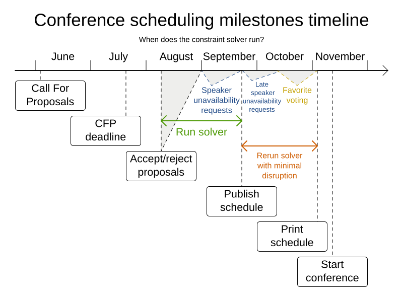
Timeslots can overlap. It reads/writes to/from an *.xlsx file that can be edited with LibreOffice or Excel.
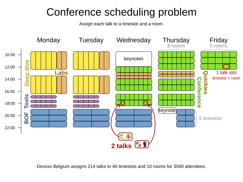
Built-in hard constraints:
-
Talk type of timeslot: The type of a talk must match the timeslot’s talk type.
-
Room unavailable timeslots: A talk’s room must be available during the talk’s timeslot.
Hard constraints (unless configured otherwise):
-
Room conflict: Two talks can’t use the same room during overlapping timeslots.
-
Speaker unavailable timeslots: Every talk’s speaker must be available during the talk’s timeslot.
-
Speaker conflict: Two talks can’t share a speaker during overlapping timeslots.
-
Talk prerequisite talks: A talk must be scheduled after all its prerequisite talks.
-
Talk mutually-exclusive-talks tags: Talks that share such tags must not be scheduled in overlapping timeslots.
-
Consecutive talks pause: A speaker who has more than one talk must have a break between them.
-
Generic purpose timeslot and room tags
-
Speaker required timeslot tags: If a speaker has a required timeslot tag, then all his/her talks must be assigned to a timeslot with that tag.
-
Speaker prohibited timeslot tags: If a speaker has a prohibited timeslot tag, then all his/her talks cannot be assigned to a timeslot with that tag.
-
Talk required timeslot tags: If a talk has a required timeslot tag, then it must be assigned to a timeslot with that tag.
-
Talk prohibited timeslot tags: If a talk has a prohibited timeslot tag, then it cannot be assigned to a timeslot with that tag.
-
Speaker required room tags: If a speaker has a required room tag, then all his/her talks must be assigned to a room with that tag.
-
Speaker prohibited room tags: If a speaker has a prohibited room tag, then all his/her talks cannot be assigned to a room with that tag.
-
Talk required room tags: If a talk has a required room tag, then it must be assigned to a room with that tag.
-
Talk prohibited room tags: If a talk has a prohibited room tag, then it cannot be assigned to a room with that tag.
-
Medium constraints (unless configured otherwise):
-
Published timeslot: A published talk must not be scheduled at a different timeslot than currently published. If a hard constraint’s input data changes after publishing (such as speaker unavailability), then this medium constraint will be minimally broken to attain a new feasible solution.
Soft constraints (unless configured otherwise):
-
Published room: Minimize the number of talks scheduled in different rooms than published ones.
-
Theme track conflict: Minimize the number of talks that share a same theme tag during overlapping timeslots.
-
Theme track room stability: Talks with common theme track tag should be scheduled in the same room throughout the day.
-
Sector conflict: Minimize the number of talks that share a same sector tag during overlapping timeslots.
-
Content audience level flow violation: For every content tag, schedule the introductory talks before the advanced talks.
-
Audience level diversity: For every timeslot, maximize the number of talks with a different audience level.
-
Language diversity: For every timeslot, maximize the number of talks with a different language.
-
Same day talks: All talks that share a theme track tag or content tag should be scheduled in the minimum number of days (ideally in the same day).
-
Popular talks: Talks with higher
favoriteCountshould be scheduled in larger rooms. -
Crowd control: Talks with higher
crowdControlRiskshould be scheduled in pairs at the same timeslot to avoid having most participants going to the same room. -
Generic purpose timeslot and room tags
-
Speaker preferred timeslot tag: If a speaker has a preferred timeslot tag, then all his/her talks should be assigned to a timeslot with that tag.
-
Speaker undesired timeslot tag: If a speaker has an undesired timeslot tag, then all his/her talks should not be assigned to a timeslot with that tag.
-
Talk preferred timeslot tag: If a talk has a preferred timeslot tag, then it should be assigned to a timeslot with that tag.
-
Talk undesired timeslot tag: If a talk has an undesired timeslot tag, then it should not be assigned to a timeslot with that tag.
-
Speaker preferred room tag: If a speaker has a preferred room tag, then all his/her talks should be assigned to a room with that tag.
-
Speaker undesired room tag: If a speaker has an undesired room tag, then all his/her talks should not be assigned to a room with that tag.
-
Talk preferred room tag: If a talk has a preferred room tag, then it should be assigned to a room with that tag.
-
Talk undesired room tag: If a talk has an undesired room tag, then it should not be assigned to a room with that tag.
-
Every constraint can be configured to use a different score level (hard/medium/soft) or a different score weight.
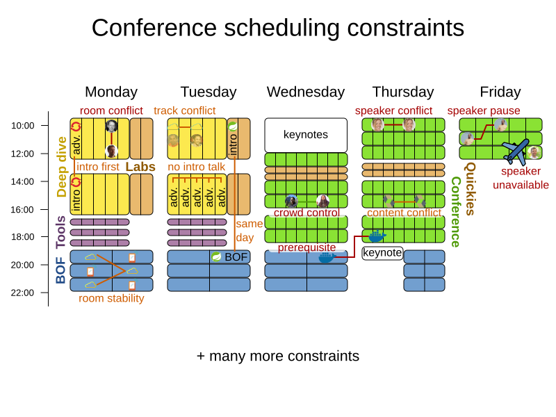
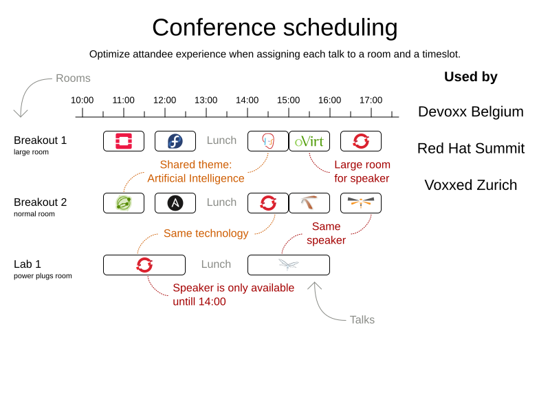
16.3. Problem size
18talks-6timeslots-5rooms    has  18 talks,  6 timeslots and  5 rooms with a search space of  10^26.
36talks-12timeslots-5rooms   has  36 talks, 12 timeslots and  5 rooms with a search space of  10^64.
72talks-12timeslots-10rooms  has  72 talks, 12 timeslots and 10 rooms with a search space of 10^149.
108talks-18timeslots-10rooms has 108 talks, 18 timeslots and 10 rooms with a search space of 10^243.
216talks-18timeslots-20rooms has 216 talks, 18 timeslots and 20 rooms with a search space of 10^552.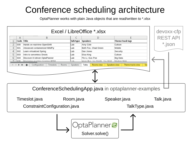
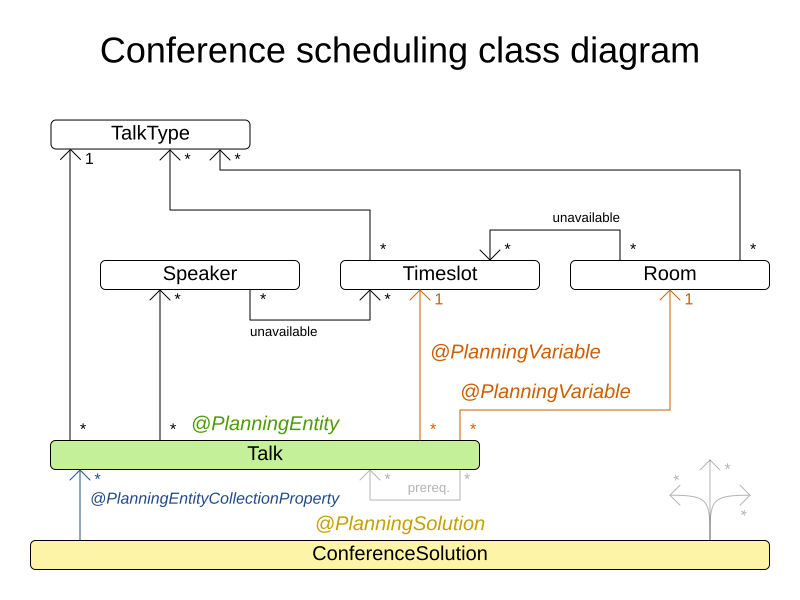
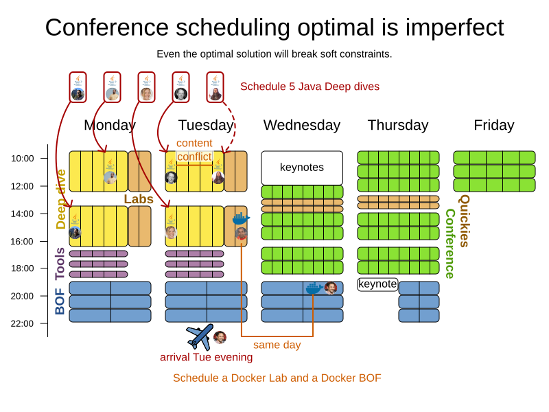
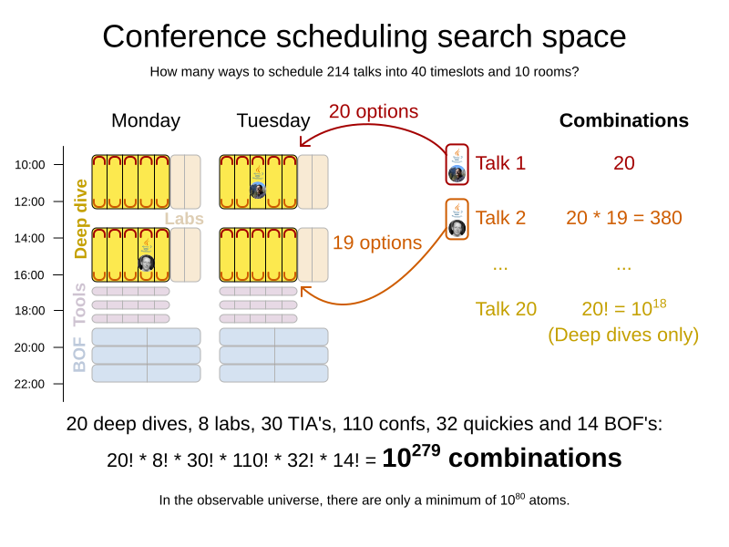
17. Flight crew scheduling
17.1. Problem description
Assign flights to pilots and flight attendants.
Hard constraints:
-
Required skill: each flight assignment has a required skill. For example, flight AB0001 requires 2 pilots and 3 flight attendants.
-
Flight conflict: each employee can only attend one flight at the same time
-
Transfer between two flights: between two flights, an employee must be able to transfer from the arrival airport to the departure airport. For example, Ann arrives in Brussels at 10:00 and departs in Amsterdam at 15:00.
-
Employee unavailability: the employee must be available on the day of the flight. For example, Ann is on vacation on 1-Feb.
Soft constraints:
-
First assignment departing from home
-
Last assignment arriving at home
-
Load balance flight duration total per employee
17.2. Problem size
175flights-7days-Europe  has 2 skills, 50 airports, 150 employees, 175 flights and  875 flight assignments with a search space of  10^1904.
700flights-28days-Europe has 2 skills, 50 airports, 150 employees, 700 flights and 3500 flight assignments with a search space of  10^7616.
875flights-7days-Europe  has 2 skills, 50 airports, 750 employees, 875 flights and 4375 flight assignments with a search space of 10^12578.
175flights-7days-US      has 2 skills, 48 airports, 150 employees, 175 flights and  875 flight assignments with a search space of  10^1904.