OptaPlanner configuration
1. Overview
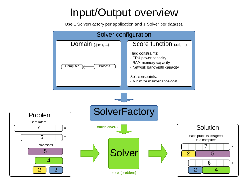
Solving a planning problem with OptaPlanner consists of the following steps:
-
Model your planning problem as a class annotated with the
@PlanningSolutionannotation, for example theNQueensclass. -
Configure a
Solver, for example a First Fit and Tabu Search solver for anyNQueensinstance. -
Load a problem data set from your data layer, for example a Four Queens instance. That is the planning problem.
-
Solve it with
Solver.solve(problem)which returns the best solution found.
2. Solver configuration
2.1. Solver configuration by XML
Build a Solver instance with the SolverFactory.
Configure the SolverFactory with a solver configuration XML file, provided as a classpath resource (as defined by ClassLoader.getResource()):
       SolverFactory<NQueens> solverFactory = SolverFactory.createFromXmlResource(
               "org/optaplanner/examples/nqueens/solver/nqueensSolverConfig.xml");
       Solver<NQueens> solver = solverFactory.buildSolver();
In a typical project (following the Maven directory structure),
that solverConfig XML file would be located at $PROJECT_DIR/src/main/resources/org/optaplanner/examples/nqueens/solver/nqueensSolverConfig.xml.
Alternatively, a SolverFactory can be created from a File with SolverFactory.createFromXmlFile().
However, for portability reasons, a classpath resource is recommended.
Both a Solver and a SolverFactory have a generic type called Solution_, which is the class representing a planning problem and solution.
A solver configuration XML file looks like this:
<?xml version="1.0" encoding="UTF-8"?>
<solver xmlns="https://www.optaplanner.org/xsd/solver" xmlns:xsi="http://www.w3.org/2001/XMLSchema-instance"
    xsi:schemaLocation="https://www.optaplanner.org/xsd/solver https://www.optaplanner.org/xsd/solver/solver.xsd">
  <!-- Define the model -->
  <solutionClass>org.optaplanner.examples.nqueens.domain.NQueens</solutionClass>
  <entityClass>org.optaplanner.examples.nqueens.domain.Queen</entityClass>

  <!-- Define the score function -->
  <scoreDirectorFactory>
    <constraintProviderClass>org.optaplanner.examples.nqueens.score.NQueensConstraintProvider</constraintProviderClass>
  </scoreDirectorFactory>

  <!-- Configure the optimization algorithms (optional) -->
  <termination>
    ...
  </termination>
  <constructionHeuristic>
    ...
  </constructionHeuristic>
  <localSearch>
    ...
  </localSearch>
</solver>
Notice the three parts in it:
-
Define the model.
-
Define the score function.
-
Optionally configure the optimization algorithm(s).
These various parts of a configuration are explained further in this manual.
OptaPlanner makes it relatively easy to switch optimization algorithm(s) just by changing the configuration. There is even a Benchmarker which allows you to play out different configurations against each other and report the most appropriate configuration for your use case.
2.2. Solver configuration by Java API
A solver configuration can also be configured with the SolverConfig API.
This is especially useful to change some values dynamically at runtime.
For example, to change the running time based on system property, before building the Solver:
        SolverConfig solverConfig = SolverConfig.createFromXmlResource(
                "org/optaplanner/examples/nqueens/solver/nqueensSolverConfig.xml");
        solverConfig.withTerminationConfig(new TerminationConfig()
                        .withMinutesSpentLimit(userInput));

        SolverFactory<NQueens> solverFactory = SolverFactory.create(solverConfig);
        Solver<NQueens> solver = solverFactory.buildSolver();
Every element in the solver configuration XML is available as a *Config class
or a property on a *Config class in the package namespace org.optaplanner.core.config.
These *Config classes are the Java representation of the XML format.
They build the runtime components (of the package namespace org.optaplanner.core.impl)
and assemble them into an efficient Solver.
|
To configure a |
2.3. Annotation alternatives
OptaPlanner needs to be told which classes in your domain model are planning entities, which properties are planning variables, etc. There are several ways to deliver this information:
-
Add class annotations and JavaBean property annotations on the domain model (recommended). The property annotations must be on the getter method, not on the setter method. Such a getter does not need to be public.
-
Add class annotations and field annotations on the domain model. Such a field does not need to be public.
-
No annotations: externalize the domain configuration in an XML file. This is not yet supported.
This manual focuses on the first manner, but every feature supports all three manners, even if it’s not explicitly mentioned.
2.4. Domain access
OptaPlanner by default accesses your domain using reflection, which will always work, but is slow compared to direct access. Alternatively, you can configure OptaPlanner to access your domain using Gizmo, which will generate bytecode that directly access the fields/methods of your domain without reflection. However, it comes with some restrictions:
-
All fields in the domain must be public.
-
The planning annotations can only be on public fields and public getters.
-
io.quarkus.gizmo:gizmo must be on the classpath.
These restrictions do not apply when using OptaPlanner with Quarkus, where Gizmo is the default domain access type.
To use Gizmo outside of Quarkus, set the domainAccessType in the
Solver Configuration:
  <solver>
    <domainAccessType>GIZMO</domainAccessType>
  </solver>
2.5. Custom properties configuration
Solver configuration elements, that instantiate classes and explicitly mention it, support custom properties.
Custom properties are useful to tweak dynamic values through the Benchmarker.
For example, presume your EasyScoreCalculator has heavy calculations (which are cached)
and you want to increase the cache size in one benchmark:
  <scoreDirectorFactory>
    <easyScoreCalculatorClass>...MyEasyScoreCalculator</easyScoreCalculatorClass>
    <easyScoreCalculatorCustomProperties>
      <property name="myCacheSize" value="1000"/><!-- Override value -->
    </easyScoreCalculatorCustomProperties>
  </scoreDirectorFactory>
Add a public setter for each custom property, which is called when a Solver is built.
public class MyEasyScoreCalculator extends EasyScoreCalculator<MySolution, SimpleScore> {

        private int myCacheSize = 500; // Default value

        @SuppressWarnings("unused")
        public void setMyCacheSize(int myCacheSize) {
            this.myCacheSize = myCacheSize;
        }

    ...
}
Most value types are supported (including boolean, int, double, BigDecimal, String and enums).
3. Model a planning problem
3.1. Is this class a problem fact or planning entity?
Look at a dataset of your planning problem. You will recognize domain classes in there, each of which can be categorized as one of the following:
-
An unrelated class: not used by any of the score constraints. From a planning standpoint, this data is obsolete.
-
A problem fact class: used by the score constraints, but does NOT change during planning (as long as the problem stays the same). For example:
Bed,Room,Shift,Employee,Topic,Period, … All the properties of a problem fact class are problem properties. -
A planning entity class: used by the score constraints and changes during planning. For example:
BedDesignation,ShiftAssignment,Exam, … The properties that change during planning are planning variables. The other properties are problem properties.
Ask yourself: What class changes during planning? Which class has variables that I want the Solver to change for me? That class is a planning entity.
Most use cases have only one planning entity class.
Most use cases also have only one planning variable per planning entity class.
|
In real-time planning, even though the problem itself changes, problem facts do not really change during planning, instead they change between planning (because the Solver temporarily stops to apply the problem fact changes). |
To create a good domain model, read the domain modeling guide.
In OptaPlanner, all problem facts and planning entities are plain old JavaBeans (POJOs). Load them from a database, an XML file, a data repository, a REST service, a noSQL cloud, … (see integration): it doesn’t matter.
3.2. Problem fact
A problem fact is any JavaBean (POJO) with getters that does not change during planning. For example in n queens, the columns and rows are problem facts:
public class Column {

    private int index;

    // ... getters
}
public class Row {
private int index;
// ... getters
}A problem fact can reference other problem facts of course:
public class Course {

    private String code;

    private Teacher teacher; // Other problem fact
    private int lectureSize;
    private int minWorkingDaySize;

    private List<Curriculum> curriculumList; // Other problem facts
    private int studentSize;

    // ... getters
}
A problem fact class does not require any OptaPlanner specific code. For example, you can reuse your domain classes, which might have JPA annotations.
|
Generally, better designed domain classes lead to simpler and more efficient score constraints.
Therefore, when dealing with a messy (denormalized) legacy system, it can sometimes be worthwhile to convert the messy domain model into a OptaPlanner specific model first.
For example: if your domain model has two Alternatively, you can sometimes also introduce a cached problem fact to enrich the domain model for planning only. |
3.3. Planning entity
3.3.1. Planning entity annotation
A planning entity is a JavaBean (POJO) that changes during solving, for example a Queen that changes to another row.
A planning problem has multiple planning entities, for example for a single n queens problem, each Queen is a planning entity.
But there is usually only one planning entity class, for example the Queen class.
A planning entity class needs to be annotated with the @PlanningEntity annotation.
Each planning entity class has one or more planning variables (which can be genuine or shadows).
It should also have one or more defining properties.
For example in n queens, a Queen is defined by its Column and has a planning variable Row.
This means that a Queen’s column never changes during solving, while its row does change.
@PlanningEntity
public class Queen {

    private Column column;

    // Planning variables: changes during planning, between score calculations.
    private Row row;

    // ... getters and setters
}
A planning entity class can have multiple planning variables.
For example, a Lecture is defined by its Course and its index in that course (because one course has multiple lectures).
Each Lecture needs to be scheduled into a Period and a Room so it has two planning variables (period and room).
For example: the course Mathematics has eight lectures per week, of which the first lecture is Monday morning at 08:00 in room 212.
@PlanningEntity
public class Lecture {

    private Course course;
    private int lectureIndexInCourse;

    // Planning variables: changes during planning, between score calculations.
    private Period period;
    private Room room;

    // ...
}
The solver configuration needs to declare each planning entity class:
<solver xmlns="https://www.optaplanner.org/xsd/solver" xmlns:xsi="http://www.w3.org/2001/XMLSchema-instance"
    xsi:schemaLocation="https://www.optaplanner.org/xsd/solver https://www.optaplanner.org/xsd/solver/solver.xsd">
  ...
  <entityClass>org.optaplanner.examples.nqueens.domain.Queen</entityClass>
  ...
</solver>
Some uses cases have multiple planning entity classes. For example: route freight and trains into railway network arcs, where each freight can use multiple trains over its journey and each train can carry multiple freights per arc. Having multiple planning entity classes directly raises the implementation complexity of your use case.
|
Do not create unnecessary planning entity classes. This leads to difficult For example, do not create a planning entity class to hold the total free time of a teacher, which needs to be kept up to date as the If historic data needs to be considered too, then create problem fact to hold the total of the historic assignments up to, but not including, the planning window (so that it does not change when a planning entity changes) and let the score constraints take it into account. |
|
Planning entity |
3.3.2. Planning entity difficulty
Some optimization algorithms work more efficiently if they have an estimation of which planning entities are more difficult to plan. For example: in bin packing bigger items are harder to fit, in course scheduling lectures with more students are more difficult to schedule, and in n queens the middle queens are more difficult to fit on the board.
|
Do not try to use planning entity difficulty to implement a business constraint. It will not affect the score function: if we have infinite solving time, the returned solution will be the same. To attain a schedule in which certain entities are scheduled earlier in the schedule, add a score constraint to change the score function so it prefers such solutions. Only consider adding planning entity difficulty too if it can make the solver more efficient. |
To allow the heuristics to take advantage of that domain specific information, set a difficultyComparatorClass to the @PlanningEntity annotation:
@PlanningEntity(difficultyComparatorClass = CloudProcessDifficultyComparator.class)
public class CloudProcess {
    // ...
}
public class CloudProcessDifficultyComparator implements Comparator<CloudProcess> {
public int compare(CloudProcess a, CloudProcess b) {
return new CompareToBuilder()
.append(a.getRequiredMultiplicand(), b.getRequiredMultiplicand())
.append(a.getId(), b.getId())
.toComparison();
}
}Alternatively, you can also set a difficultyWeightFactoryClass to the @PlanningEntity annotation,
so that you have access to the rest of the problem facts from the solution too:
@PlanningEntity(difficultyWeightFactoryClass = QueenDifficultyWeightFactory.class)
public class Queen {
    // ...
}
See sorted selection for more information.
|
Difficulty should be implemented ascending: easy entities are lower, difficult entities are higher. For example, in bin packing: small item < medium item < big item. Although most algorithms start with the more difficult entities first, they just reverse the ordering. |
None of the current planning variable states should be used to compare planning entity difficulty. During Construction Heuristics, those variables are likely to be null anyway.
For example, a Queen's row variable should not be used.
3.4. Planning variable (genuine)
3.4.1. Planning variable annotation
A planning variable is a JavaBean property (so a getter and setter) on a planning entity.
It points to a planning value, which changes during planning.
For example, a Queen's row property is a genuine planning variable.
Note that even though a Queen's row property changes to another Row during planning, no Row instance itself is changed.
Normally planning variables are genuine, but advanced cases can also have shadows.
A genuine planning variable getter needs to be annotated with the @PlanningVariable annotation, optionally with a non-empty valueRangeProviderRefs property.
@PlanningEntity
public class Queen {
    ...

    private Row row;

    @PlanningVariable
    public Row getRow() {
        return row;
    }

    public void setRow(Row row) {
        this.row = row;
    }

}
The optional valueRangeProviderRefs property defines what are the possible planning values for this planning variable.
It references one or more @ValueRangeProvider id's.
If none are provided, OptaPlanner will attempt to auto-detect matching @ValueRangeProviders.
|
A @PlanningVariable annotation needs to be on a member in a class with a @PlanningEntity annotation. It is ignored on parent classes or subclasses without that annotation. |
Annotating the field instead of the property works too:
@PlanningEntity
public class Queen {
    ...

    @PlanningVariable
    private Row row;

}|
For more advanced planning variables used to model precedence relationships, see planning list variable and chained planning variable. |
3.4.2. Nullable planning variable
By default, an initialized planning variable cannot be null, so an initialized solution will never use null for any of its planning variables.
In an over-constrained use case, this can be counterproductive.
For example: in task assignment with too many tasks for the workforce, we would rather leave low priority tasks unassigned instead of assigning them to an overloaded worker.
To allow an initialized planning variable to be null, set nullable to true:
    @PlanningVariable(..., nullable = true)
    public Worker getWorker() {
        return worker;
}|
Constraint Streams filter out planning entities with a |
OptaPlanner will automatically add the value null to the value range.
There is no need to add null in a collection provided by a ValueRangeProvider.
|
Using a nullable planning variable implies that your score calculation is responsible for punishing (or even rewarding) variables with a |
|
Currently chained planning variables are not compatible with |
Repeated planning (especially real-time planning) does not mix well with a nullable planning variable.
Every time the Solver starts or a problem fact change is made, the Construction Heuristics
will try to initialize all the null variables again, which can be a huge waste of time.
One way to deal with this is to filter the entity selector of the placer in the construction heuristic.
<solver xmlns="https://www.optaplanner.org/xsd/solver" xmlns:xsi="http://www.w3.org/2001/XMLSchema-instance"
    xsi:schemaLocation="https://www.optaplanner.org/xsd/solver https://www.optaplanner.org/xsd/solver/solver.xsd">
  ...
  <constructionHeuristic>
    <queuedEntityPlacer>
      <entitySelector id="entitySelector1">
        <filterClass>...</filterClass>
      </entitySelector>
    </queuedEntityPlacer>
    ...
    <changeMoveSelector>
      <entitySelector mimicSelectorRef="entitySelector1" />
    </changeMoveSelector>
    ...
  </constructionHeuristic>
 ...
</solver>
3.4.3. When is a planning variable considered initialized?
A planning variable is considered initialized if its value is not null or if the variable is nullable.
So a nullable variable is always considered initialized.
A planning entity is initialized if all of its planning variables are initialized.
A solution is initialized if all of its planning entities are initialized.
3.5. Planning value and planning value range
3.5.1. Planning value
A planning value is a possible value for a genuine planning variable.
Usually, a planning value is a problem fact, but it can also be any object, for example a double.
It can even be another planning entity or even an interface implemented by both a planning entity and a problem fact.
A planning value range is the set of possible planning values for a planning variable.
This set can be a countable (for example row 1, 2, 3 or 4) or uncountable (for example any double between 0.0 and 1.0).
3.5.2. Planning value range provider
Overview
The value range of a planning variable is defined with the @ValueRangeProvider annotation.
A @ValueRangeProvider may carry a property id, which is referenced by the @PlanningVariable's property valueRangeProviderRefs.
This annotation can be located on two types of methods:
-
On the Solution: All planning entities share the same value range.
-
On the planning entity: The value range differs per planning entity. This is less common.
|
A @ValueRangeProvider annotation needs to be on a member in a class with a @PlanningSolution or a @PlanningEntity annotation. It is ignored on parent classes or subclasses without those annotations. |
The return type of that method can be three types:
-
Collection: The value range is defined by aCollection(usually aList) of its possible values. -
Array: The value range is defined by an array of its possible values.
-
ValueRange: The value range is defined by its bounds. This is less common.
ValueRangeProvider on the solution
All instances of the same planning entity class share the same set of possible planning values for that planning variable. This is the most common way to configure a value range.
The @PlanningSolution implementation has method that returns a Collection (or a ValueRange).
Any value from that Collection is a possible planning value for this planning variable.
    @PlanningVariable
    public Row getRow() {
        return row;
    }
@PlanningSolution
public class NQueens {
...
@ValueRangeProvider
public List<Row> getRowList() {
return rowList;
}
}|
That |
Annotating the field instead of the property works too:
@PlanningSolution
public class NQueens {
    ...

    @ValueRangeProvider
    private List<Row> rowList;

}
ValueRangeProvider on the Planning Entity
Each planning entity has its own value range (a set of possible planning values) for the planning variable. For example, if a teacher can never teach in a room that does not belong to his department, lectures of that teacher can limit their room value range to the rooms of his department.
    @PlanningVariable
    public Room getRoom() {
        return room;
    }

    @ValueRangeProvider
    public List<Room> getPossibleRoomList() {
        return getCourse().getTeacher().getDepartment().getRoomList();
    }
Never use this to enforce a soft constraint (or even a hard constraint when the problem might not have a feasible solution). For example: Unless there is no other way, a teacher cannot teach in a room that does not belong to his department. In this case, the teacher should not be limited in his room value range (because sometimes there is no other way).
|
By limiting the value range specifically of one planning entity, you are effectively creating a built-in hard constraint. This can have the benefit of severely lowering the number of possible solutions; however, it can also take away the freedom of the optimization algorithms to temporarily break that constraint in order to escape from a local optimum. |
A planning entity should not use other planning entities to determine its value range. That would only try to make the planning entity solve the planning problem itself and interfere with the optimization algorithms.
Every entity has its own List instance, unless multiple entities have the same value range.
For example, if teacher A and B belong to the same department, they use the same List<Room> instance.
Furthermore, each List contains a subset of the same set of planning value instances.
For example, if department A and B can both use room X, then their List<Room> instances contain the same Room instance.
|
A |
|
A |
|
A |
Referencing ValueRangeProviders
There are two ways how to match a planning variable to a value range provider. The simplest way is to have value range provider auto-detected. Another way is to explicitly reference the value range provider.
Anonymous ValueRangeProviders
We already described the first approach.
By not providing any valueRangeProviderRefs on the @PlanningVariable annotation,
OptaPlanner will go over every @ValueRangeProvider-annotated method or field which does not have an id property set,
and will match planning variables with value ranges where their types match.
In the following example,
the planning variable car will be matched to the value range returned by getCompanyCarList(),
as they both use the Car type.
It will not match getPersonalCarList(),
because that value range provider is not anonymous; it specifies an id.
    @PlanningVariable
    public Car getCar() {
        return car;
    }

    @ValueRangeProvider
    public List<Car> getCompanyCarList() {
        return companyCarList;
    }

    @ValueRangeProvider(id = "personalCarRange")
    public List<Car> getPersonalCarList() {
        return personalCarList;
    }
Automatic matching also accounts for polymorphism.
In the following example,
the planning variable car will be matched to getCompanyCarList() and getPersonalCarList(),
as both CompanyCar and PersonalCar are Cars.
It will not match getAirplanes(),
as an Airplane is not a Car.
    @PlanningVariable
    public Car getCar() {
        return car;
    }

    @ValueRangeProvider
    public List<CompanyCar> getCompanyCarList() {
        return companyCarList;
    }

    @ValueRangeProvider
    public List<PersonalCar> getPersonalCarList() {
        return personalCarList;
    }

    @ValueRangeProvider
    public List<Airplane> getAirplanes() {
        return airplaneList;
    }
Explicitly referenced ValueRangeProviders
In more complicated cases where auto-detection is not sufficient or where clarity is preferred over simplicity, value range providers can also be referenced explicitly.
In the following example,
the car planning variable will only be matched to value range provided by methods getCompanyCarList().
    @PlanningVariable(valueRangeProviderRefs = {"companyCarRange"})
    public Car getCar() {
        return car;
    }

    @ValueRangeProvider(id = "companyCarRange")
    public List<CompanyCar> getCompanyCarList() {
        return companyCarList;
    }

    @ValueRangeProvider(id = "personalCarRange")
    public List<PersonalCar> getPersonalCarList() {
        return personalCarList;
    }
Explicitly referenced value range providers can also be combined, for example:
    @PlanningVariable(valueRangeProviderRefs = { "companyCarRange", "personalCarRange" })
    public Car getCar() {
        return car;
    }

    @ValueRangeProvider(id = "companyCarRange")
    public List<CompanyCar> getCompanyCarList() {
        return companyCarList;
    }

    @ValueRangeProvider(id = "personalCarRange")
    public List<PersonalCar> getPersonalCarList() {
        return personalCarList;
    }
ValueRangeFactory
Instead of a Collection, you can also return a ValueRange or CountableValueRange, built by the ValueRangeFactory:
    @ValueRangeProvider
    public CountableValueRange<Integer> getDelayRange() {
        return ValueRangeFactory.createIntValueRange(0, 5000);
    }
A ValueRange uses far less memory, because it only holds the bounds.
In the example above, a Collection would need to hold all 5000 ints, instead of just the two bounds.
Furthermore, an incrementUnit can be specified, for example if you have to buy stocks in units of 200 pieces:
    @ValueRangeProvider
    public CountableValueRange<Integer> getStockAmountRange() {
         // Range: 0, 200, 400, 600, ..., 9999600, 9999800, 10000000
        return ValueRangeFactory.createIntValueRange(0, 10000000, 200);
}|
Return |
The ValueRangeFactory has creation methods for several value class types:
-
boolean: A boolean range. -
int: A 32bit integer range. -
long: A 64bit integer range. -
double: A 64bit floating point range which only supports random selection (because it does not implementCountableValueRange). -
BigInteger: An arbitrary-precision integer range. -
BigDecimal: A decimal point range. By default, the increment unit is the lowest non-zero value in the scale of the bounds. -
Temporal(such asLocalDate,LocalDateTime, …): A time range.
3.5.3. Planning value strength
Some optimization algorithms work a bit more efficiently if they have an estimation of which planning values are stronger, which means they are more likely to satisfy a planning entity. For example: in bin packing bigger containers are more likely to fit an item and in course scheduling bigger rooms are less likely to break the student capacity constraint. Usually, the efficiency gain of planning value strength is far less than that of planning entity difficulty.
|
Do not try to use planning value strength to implement a business constraint. It will not affect the score function: if we have infinite solving time, the returned solution will be the same. To affect the score function, add a score constraint. Only consider adding planning value strength too if it can make the solver more efficient. |
To allow the heuristics to take advantage of that domain specific information, set a strengthComparatorClass to the @PlanningVariable annotation:
    @PlanningVariable(..., strengthComparatorClass = CloudComputerStrengthComparator.class)
    public CloudComputer getComputer() {
        return computer;
    }
public class CloudComputerStrengthComparator implements Comparator<CloudComputer> {
public int compare(CloudComputer a, CloudComputer b) {
return new CompareToBuilder()
.append(a.getMultiplicand(), b.getMultiplicand())
.append(b.getCost(), a.getCost()) // Descending (but this is debatable)
.append(a.getId(), b.getId())
.toComparison();
}
}|
If you have multiple planning value classes in the same value range, the |
Alternatively, you can also set a strengthWeightFactoryClass to the @PlanningVariable annotation, so you have access to the rest of the problem facts from the solution too:
    @PlanningVariable(..., strengthWeightFactoryClass = RowStrengthWeightFactory.class)
    public Row getRow() {
        return row;
    }
See sorted selection for more information.
|
Strength should be implemented ascending: weaker values are lower, stronger values are higher. For example in bin packing: small container < medium container < big container. |
None of the current planning variable state in any of the planning entities should be used to compare planning values. During construction heuristics, those variables are likely to be null.
For example, none of the row variables of any Queen may be used to determine the strength of a Row.
3.6. Planning list variable (VRP, Task assigning, …)
Use the planning list variable to model problems where the goal is to distribute a number of workload elements among limited resources in a specific order. This includes, for example, vehicle routing, traveling salesman, task assigning, and similar problems, that have previously been modeled using the chained planning variable.
The planning list variable is a successor to the chained planning variable and provides a more intuitive way to express the problem domain with Java classes.
|
As a new feature, planning list variable does not yet support all the advanced planning features that work with the chained planning variable. Use a chained planning variable instead of a planning list variable, if you need any of the following planning techniques:
|
For example, the vehicle routing problem can be modeled as follows:
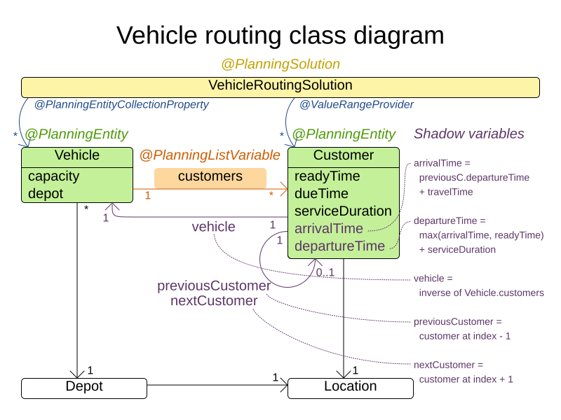
This model is closer to the reality than the chained model. Each vehicle has a list of customers to go to in the order given by the list. And indeed, the object model matches the natural language description of the problem:
@PlanningEntity
class Vehicle {

    int capacity;
    Depot depot;

    @PlanningListVariable
    List<Customer> customers = new ArrayList<>();
}
Planning list variable can be used if the domain meets the following criteria:
-
There is a one-to-many relationship between the planning entity and the planning value.
-
The order in which planning values are assigned to an entity’s list variable is significant.
-
Each planning value is assigned to exactly one planning entity. No planning value may appear in multiple entities.
3.7. Chained planning variable (TSP, VRP, …)
Chained planning variable is one way to implement the Chained Through Time pattern. This pattern is used for some use cases, such as TSP and vehicle routing. Use the chained planning variable to implement this pattern if you plan to use some of the advanced planning features, that are not yet supported by the planning list variable.
Chained planning variable allows the planning entities to point to each other and form a chain. By modeling the problem as a set of chains (instead of a set of trees/loops), the search space is heavily reduced.
A planning variable that is chained either:
-
Directly points to a problem fact (or planning entity), which is called an anchor.
-
Points to another planning entity with the same planning variable, which recursively points to an anchor.
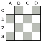
Here are some examples of valid and invalid chains:
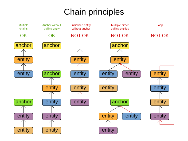
Every initialized planning entity is part of an open-ended chain that begins from an anchor. A valid model means that:
-
A chain is never a loop. The tail is always open.
-
Every chain always has exactly one anchor. The anchor is never an instance of the planning entity class that contains the chained planning variable.
-
A chain is never a tree, it is always a line. Every anchor or planning entity has at most one trailing planning entity.
-
Every initialized planning entity is part of a chain.
-
An anchor with no planning entities pointing to it, is also considered a chain.
|
A planning problem instance given to the |
|
If your constraints dictate a closed chain, model it as an open-ended chain (which is easier to persist in a database) and implement a score constraint for the last entity back to the anchor. |
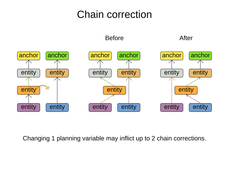
The optimization algorithms and built-in Moves do chain correction to guarantee that the model stays valid:
|
A custom |
For example, in TSP the anchor is a Domicile (in vehicle routing it is Vehicle):
public class Domicile ... implements Standstill {
    ...

    public City getCity() {...}

}
The anchor (which is a problem fact) and the planning entity implement a common interface, for example TSP’s Standstill:
public interface Standstill {

    City getCity();

}
That interface is the return type of the planning variable.
Furthermore, the planning variable is chained.
For example TSP’s Visit:
@PlanningEntity
public class Visit ... implements Standstill {
    ...

    public City getCity() {...}

    @PlanningVariable(graphType = PlanningVariableGraphType.CHAINED)
    public Standstill getPreviousStandstill() {
        return previousStandstill;
    }

    public void setPreviousStandstill(Standstill previousStandstill) {
        this.previousStandstill = previousStandstill;
    }

}
Notice how two value range providers are usually combined:
-
The value range provider that holds the anchors, for example
domicileList. -
The value range provider that holds the initialized planning entities, for example
visitList.
3.8. Planning problem and planning solution
3.8.1. Planning problem instance
A dataset for a planning problem needs to be wrapped in a class for the Solver to solve.
That solution class represents both the planning problem and (if solved) a solution.
It is annotated with a @PlanningSolution annotation.
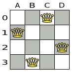
For example in n queens, the solution class is the NQueens class, which contains a Column list, a Row list, and a Queen list.
A planning problem is actually an unsolved planning solution or - stated differently - an uninitialized solution.
For example in n queens, that NQueens class has the @PlanningSolution annotation, yet every Queen in an unsolved NQueens class is not yet assigned to a Row (their row property is null). That’s not a feasible solution.
It’s not even a possible solution.
It’s an uninitialized solution.
3.8.2. Solution class
A solution class holds all problem facts, planning entities and a score.
It is annotated with a @PlanningSolution annotation.
For example, an NQueens instance holds a list of all columns, all rows and all Queen instances:
@PlanningSolution
public class NQueens {

    // Problem facts
    private int n;
    private List<Column> columnList;
    private List<Row> rowList;

    // Planning entities
    private List<Queen> queenList;

    private SimpleScore score;

    ...
}
The solver configuration needs to declare the planning solution class:
<solver xmlns="https://www.optaplanner.org/xsd/solver" xmlns:xsi="http://www.w3.org/2001/XMLSchema-instance"
    xsi:schemaLocation="https://www.optaplanner.org/xsd/solver https://www.optaplanner.org/xsd/solver/solver.xsd">
  ...
  <solutionClass>org.optaplanner.examples.nqueens.domain.NQueens</solutionClass>
  ...
</solver>
3.8.3. Planning entities of a solution (@PlanningEntityCollectionProperty)
OptaPlanner needs to extract the entity instances from the solution instance.
It gets those collection(s) by calling every getter (or field) that is annotated with @PlanningEntityCollectionProperty:
@PlanningSolution
public class NQueens {
    ...

    private List<Queen> queenList;

    @PlanningEntityCollectionProperty
    public List<Queen> getQueenList() {
        return queenList;
    }

}
There can be multiple @PlanningEntityCollectionProperty annotated members.
Those can even return a Collection with the same entity class type.
Instead of Collection, it can also return an array.
|
A |
In rare cases, a planning entity might be a singleton: use @PlanningEntityProperty on its getter (or field) instead.
Both annotations can also be auto discovered if enabled.
3.8.4. Score of a Solution (@PlanningScore)
A @PlanningSolution class requires a score property (or field), which is annotated with a @PlanningScore annotation.
The score property is null if the score hasn’t been calculated yet.
The score property is typed to the specific Score implementation of your use case.
For example, NQueens uses a SimpleScore:
@PlanningSolution
public class NQueens {
    ...

    private SimpleScore score;

    @PlanningScore
    public SimpleScore getScore() {
        return score;
    }
    public void setScore(SimpleScore score) {
        this.score = score;
    }

}
Most use cases use a HardSoftScore instead:
@PlanningSolution
public class CloudBalance {
    ...

    private HardSoftScore score;

    @PlanningScore
    public HardSoftScore getScore() {
        return score;
    }

    public void setScore(HardSoftScore score) {
        this.score = score;
    }

}
Some use cases use other score types.
This annotation can also be auto discovered if enabled.
3.8.5. Problem facts of a solution (@ProblemFactCollectionProperty)
For Constraint Streams and Drools score calculation (Deprecated),
OptaPlanner needs to extract the problem fact instances from the solution instance.
It gets those collection(s) by calling every method (or field) that is annotated with @ProblemFactCollectionProperty.
All objects returned by those methods are available to use by Constraint Streams or Drools rules.
For example in NQueens all Column and Row instances are problem facts.
@PlanningSolution
public class NQueens {
    ...

    private List<Column> columnList;
    private List<Row> rowList;

    @ProblemFactCollectionProperty
    public List<Column> getColumnList() {
        return columnList;
    }

    @ProblemFactCollectionProperty
    public List<Row> getRowList() {
        return rowList;
    }

}
All planning entities are automatically inserted into the working memory. Do not add an annotation on their properties.
|
The problem facts methods are not called often: at most only once per solver phase per solver thread. |
There can be multiple @ProblemFactCollectionProperty annotated members.
Those can even return a Collection with the same class type, but they shouldn’t return the same instance twice.
Instead of Collection, it can also return an array.
|
A @ProblemFactCollectionProperty annotation needs to be on a member in a class with a @PlanningSolution annotation. It is ignored on parent classes or subclasses without that annotation. |
In rare cases, a problem fact might be a singleton: use @ProblemFactProperty on its method (or field) instead.
Both annotations can also be auto discovered if enabled.
Cached problem fact
A cached problem fact is a problem fact that does not exist in the real domain model, but is calculated before the Solver really starts solving.
The problem facts methods have the opportunity to enrich the domain model with such cached problem facts, which can lead to simpler and faster score constraints.
For example in examination, a cached problem fact TopicConflict is created for every two Topics which share at least one Student.
    @ProblemFactCollectionProperty
    private List<TopicConflict> calculateTopicConflictList() {
        List<TopicConflict> topicConflictList = new ArrayList<TopicConflict>();
        for (Topic leftTopic : topicList) {
            for (Topic rightTopic : topicList) {
                if (leftTopic.getId() < rightTopic.getId()) {
                    int studentSize = 0;
                    for (Student student : leftTopic.getStudentList()) {
                        if (rightTopic.getStudentList().contains(student)) {
                            studentSize++;
                        }
                    }
                    if (studentSize > 0) {
                        topicConflictList.add(new TopicConflict(leftTopic, rightTopic, studentSize));
                    }
                }
            }
        }
        return topicConflictList;
    }
Where a score constraint needs to check that no two exams with a topic that shares a student are scheduled close together (depending on the constraint: at the same time, in a row, or in the same day), the TopicConflict instance can be used as a problem fact, rather than having to combine every two Student instances.
3.8.6. Auto discover solution properties
Instead of configuring each property (or field) annotation explicitly, some can also be deduced automatically by OptaPlanner. For example, on the cloud balancing example:
@PlanningSolution(autoDiscoverMemberType = AutoDiscoverMemberType.FIELD)
public class CloudBalance {

    // Auto discovered as @ProblemFactCollectionProperty
    @ValueRangeProvider
    private List<CloudComputer> computerList;

    // Auto discovered as @PlanningEntityCollectionProperty
    private List<CloudProcess> processList;

    // Auto discovered as @PlanningScore
    private HardSoftScore score;

    ...
}
The AutoDiscoverMemberType can be:
-
NONE: No auto discovery. -
FIELD: Auto discover all fields on the@PlanningSolutionclass -
GETTER: Auto discover all getters on the@PlanningSolutionclass
The automatic annotation is based on the field type (or getter return type):
-
@ProblemFactProperty: when it isn’t aCollection, an array, a@PlanningEntityclass or aScore -
@ProblemFactCollectionProperty: when it’s aCollection(or array) of a type that isn’t a@PlanningEntityclass -
@PlanningEntityProperty: when it is a configured@PlanningEntityclass or subclass -
@PlanningEntityCollectionProperty: when it’s aCollection(or array) of a type that is a configured@PlanningEntityclass or subclass -
@PlanningScore: when it is aScoreor subclass
These automatic annotations can still be overwritten per field (or getter).
Specifically, a BendableScore always needs to override
with an explicit @PlanningScore annotation to define the number of hard and soft levels.
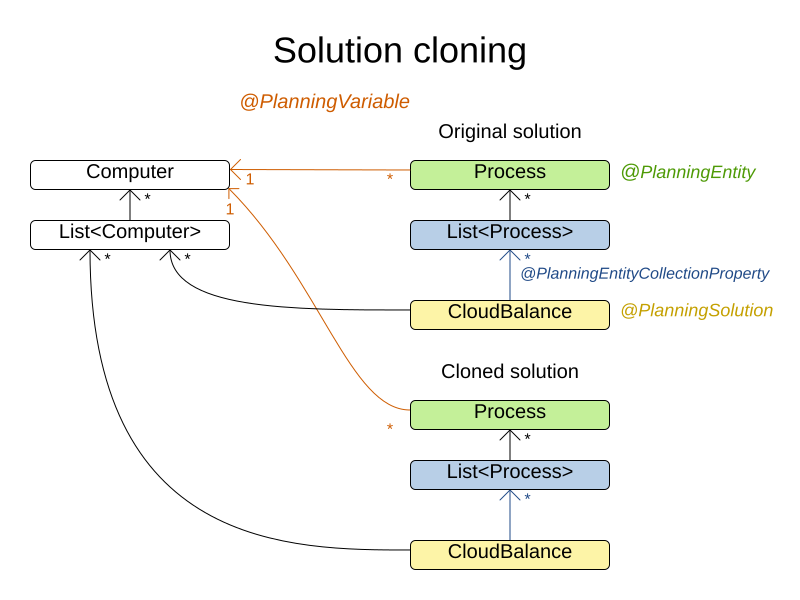
3.8.7. Cloning a solution
Most (if not all) optimization algorithms clone the solution each time they encounter a new best solution (so they can recall it later) or to work with multiple solutions in parallel.
|
There are many ways to clone, such as a shallow clone, deep clone, … This context focuses on a planning clone. |
A planning clone of a solution must fulfill these requirements:
-
The clone must represent the same planning problem. Usually it reuses the same instances of the problem facts and problem fact collections as the original.
-
The clone must use different, cloned instances of the entities and entity collections. Changes to an original solution entity’s variables must not affect its clone.
Implementing a planning clone method is hard, therefore you do not need to implement it.
FieldAccessingSolutionCloner
This SolutionCloner is used by default.
It works well for most use cases.
|
When the |
The FieldAccessingSolutionCloner does not clone problem facts by default.
If any of your problem facts needs to be deep cloned for a planning clone,
for example if the problem fact references a planning entity or the planning solution,
mark its class with a @DeepPlanningClone annotation:
@DeepPlanningClone
public class SeatDesignationDependency {
    private SeatDesignation leftSeatDesignation; // planning entity
    private SeatDesignation rightSeatDesignation; // planning entity
    ...
}
In the example above, because SeatDesignationDependency references the planning entity SeatDesignation
(which is deep planning cloned automatically), it should also be deep planning cloned.
Alternatively, the @DeepPlanningClone annotation also works on a getter method or a field to planning clone it.
If that property is a Collection or a Map, it will shallow clone it and deep planning clone
any element thereof that is an instance of a class that has a @DeepPlanningClone annotation.
Custom cloning with a SolutionCloner
To use a custom cloner, configure it on the planning solution:
@PlanningSolution(solutionCloner = NQueensSolutionCloner.class)
public class NQueens {
    ...
}
For example, a NQueens planning clone only deep clones all Queen instances.
So when the original solution changes (later on during planning) and one or more Queen instances change,
the planning clone isn’t affected.
public class NQueensSolutionCloner implements SolutionCloner<NQueens> {

    @Override
    public NQueens cloneSolution(CloneLedger ledger, NQueens original) {
        NQueens clone = new NQueens();
        ledger.registerClone(original, clone);
        clone.setId(original.getId());
        clone.setN(original.getN());
        clone.setColumnList(original.getColumnList());
        clone.setRowList(original.getRowList());
        List<Queen> queenList = original.getQueenList();
        List<Queen> clonedQueenList = new ArrayList<Queen>(queenList.size());
        for (Queen originalQueen : queenList) {
            Queen cloneQueen = new Queen();
            ledger.registerClone(originalQueen, cloneQueen);
            cloneQueen.setId(originalQueen.getId());
            cloneQueen.setColumn(originalQueen.getColumn());
            cloneQueen.setRow(originalQueen.getRow());
            clonedQueenList.add(cloneQueen);
        }
        clone.setQueenList(clonedQueenList);
        clone.setScore(original.getScore());
        return clone;
    }

}
The cloneSolution() method should only deep clone the planning entities.
Notice that the problem facts, such as Column and Row are normally not cloned: even their List instances are not cloned.
If the problem facts were cloned too, then you would have to make sure that the new planning entity clones also refer to the new problem facts clones used by the cloned solution.
For example, if you were to clone all Row instances, then each Queen clone and the NQueens clone itself should refer to those new Row clones.
|
Cloning an entity with a chained variable is devious: a variable of an entity A might point to another entity B. If A is cloned, then its variable must point to the clone of B, not the original B. |
3.8.8. Create an uninitialized solution
Create a @PlanningSolution instance to represent your planning problem’s dataset, so it can be set on the Solver as the planning problem to solve.
For example in n queens, an NQueens instance is created with the required Column and Row instances and every Queen set to a different column and every row set to null.
    private NQueens createNQueens(int n) {
        NQueens nQueens = new NQueens();
        nQueens.setId(0L);
        nQueens.setN(n);
        nQueens.setColumnList(createColumnList(nQueens));
        nQueens.setRowList(createRowList(nQueens));
        nQueens.setQueenList(createQueenList(nQueens));
        return nQueens;
    }

    private List<Queen> createQueenList(NQueens nQueens) {
        int n = nQueens.getN();
        List<Queen> queenList = new ArrayList<Queen>(n);
        long id = 0L;
        for (Column column : nQueens.getColumnList()) {
            Queen queen = new Queen();
            queen.setId(id);
            id++;
            queen.setColumn(column);
            // Notice that we leave the PlanningVariable properties on null
            queenList.add(queen);
        }
        return queenList;
    }
Usually, most of this data comes from your data layer, and your solution implementation just aggregates that data and creates the uninitialized planning entity instances to plan:
        private void createLectureList(CourseSchedule schedule) {
            List<Course> courseList = schedule.getCourseList();
            List<Lecture> lectureList = new ArrayList<Lecture>(courseList.size());
            long id = 0L;
            for (Course course : courseList) {
                for (int i = 0; i < course.getLectureSize(); i++) {
                    Lecture lecture = new Lecture();
                    lecture.setId(id);
                    id++;
                    lecture.setCourse(course);
                    lecture.setLectureIndexInCourse(i);
                    // Notice that we leave the PlanningVariable properties (period and room) on null
                    lectureList.add(lecture);
                }
            }
            schedule.setLectureList(lectureList);
        }
4. Use the Solver
4.1. The Solver interface
A Solver solves your planning problem.
public interface Solver<Solution_> {

    Solution_ solve(Solution_ problem);

    ...
}
A Solver can only solve one planning problem instance at a time.
It is built with a SolverFactory, there is no need to implement it yourself.
A Solver should only be accessed from a single thread, except for the methods that are specifically documented in javadoc as being thread-safe.
The solve() method hogs the current thread.
This can cause HTTP timeouts for REST services and it requires extra code to solve multiple datasets in parallel.
To avoid such issues, use a SolverManager instead.
4.2. Solving a problem
Solving a problem is quite easy once you have:
-
A
Solverbuilt from a solver configuration -
A
@PlanningSolutionthat represents the planning problem instance
Just provide the planning problem as argument to the solve() method and it will return the best solution found:
    NQueens problem = ...;
    NQueens bestSolution = solver.solve(problem);
For example in n queens, the solve() method will return an NQueens instance with every Queen assigned to a Row.
The solve(Solution) method can take a long time (depending on the problem size and the solver configuration). The Solver intelligently wades through the search space of possible solutions and remembers the best solution it encounters during solving.
Depending on a number of factors (including problem size, how much time the Solver has, the solver configuration, …), that best solution might or might not be an optimal solution.
|
The solution instance given to the method The solution instance returned by the methods |
|
The solution instance given to the |
4.3. Environment mode: are there bugs in my code?
The environment mode allows you to detect common bugs in your implementation. It does not affect the logging level.
You can set the environment mode in the solver configuration XML file:
<solver xmlns="https://www.optaplanner.org/xsd/solver" xmlns:xsi="http://www.w3.org/2001/XMLSchema-instance"
    xsi:schemaLocation="https://www.optaplanner.org/xsd/solver https://www.optaplanner.org/xsd/solver/solver.xsd">
  <environmentMode>FAST_ASSERT</environmentMode>
  ...
</solver>
A solver has a single Random instance.
Some solver configurations use the Random instance a lot more than others.
For example, Simulated Annealing depends highly on random numbers, while Tabu Search only depends on it to deal with score ties.
The environment mode influences the seed of that Random instance.
These are the environment modes:
4.3.1. FULL_ASSERT
The FULL_ASSERT mode turns on all assertions (such as assert that the incremental score calculation is uncorrupted for each move) to fail-fast on a bug in a Move implementation, a constraint, the engine itself, …
This mode is reproducible (see the reproducible mode). It is also intrusive because it calls the method calculateScore() more frequently than a non-assert mode.
The FULL_ASSERT mode is horribly slow (because it does not rely on incremental score calculation).
4.3.2. NON_INTRUSIVE_FULL_ASSERT
The NON_INTRUSIVE_FULL_ASSERT turns on several assertions to fail-fast on a bug in a Move implementation, a constraint, the engine itself, …
This mode is reproducible (see the reproducible mode). It is non-intrusive because it does not call the method calculateScore() more frequently than a non assert mode.
The NON_INTRUSIVE_FULL_ASSERT mode is horribly slow (because it does not rely on incremental score calculation).
4.3.3. FAST_ASSERT
The FAST_ASSERT mode turns on most assertions (such as assert that an undoMove’s score is the same as before the Move) to fail-fast on a bug in a Move implementation, a constraint, the engine itself, …
This mode is reproducible (see the reproducible mode). It is also intrusive because it calls the method calculateScore() more frequently than a non assert mode.
The FAST_ASSERT mode is slow.
It is recommended to write a test case that does a short run of your planning problem with the FAST_ASSERT mode on.
4.3.4. REPRODUCIBLE (default)
The reproducible mode is the default mode because it is recommended during development. In this mode, two runs in the same OptaPlanner version will execute the same code in the same order. Those two runs will have the same result at every step, except if the note below applies. This enables you to reproduce bugs consistently. It also allows you to benchmark certain refactorings (such as a score constraint performance optimization) fairly across runs.
|
Despite the reproducible mode, your application might still not be fully reproducible because of:
|
The reproducible mode can be slightly slower than the non-reproducible mode. If your production environment can benefit from reproducibility, use this mode in production.
In practice, this mode uses the default, fixed random seed if no seed is specified, and it also disables certain concurrency optimizations (such as work stealing).
4.3.5. NON_REPRODUCIBLE
The non-reproducible mode can be slightly faster than the reproducible mode. Avoid using it during development as it makes debugging and bug fixing painful. If your production environment doesn’t care about reproducibility, use this mode in production.
In practice, this mode uses no fixed random seed if no seed is specified.
4.4. Logging level: what is the Solver doing?
The best way to illuminate the black box that is a Solver, is to play with the logging level:
-
error: Log errors, except those that are thrown to the calling code as a
RuntimeException.If an error happens, OptaPlanner normally fails fast: it throws a subclass of
RuntimeExceptionwith a detailed message to the calling code. It does not log it as an error itself to avoid duplicate log messages. Except if the calling code explicitly catches and eats thatRuntimeException, aThread's defaultExceptionHandlerwill log it as an error anyway. Meanwhile, the code is disrupted from doing further harm or obfuscating the error. -
warn: Log suspicious circumstances.
-
info: Log every phase and the solver itself. See scope overview.
-
debug: Log every step of every phase. See scope overview.
-
trace: Log every move of every step of every phase. See scope overview.
|
Turning on Even Both cause congestion in multithreaded solving with most appenders, see below. In Eclipse, |
For example, set it to debug logging, to see when the phases end and how fast steps are taken:
INFO  Solving started: time spent (3), best score (-4init/0), random (JDK with seed 0).
DEBUG     CH step (0), time spent (5), score (-3init/0), selected move count (1), picked move (Queen-2 {null -> Row-0}).
DEBUG     CH step (1), time spent (7), score (-2init/0), selected move count (3), picked move (Queen-1 {null -> Row-2}).
DEBUG     CH step (2), time spent (10), score (-1init/0), selected move count (4), picked move (Queen-3 {null -> Row-3}).
DEBUG     CH step (3), time spent (12), score (-1), selected move count (4), picked move (Queen-0 {null -> Row-1}).
INFO  Construction Heuristic phase (0) ended: time spent (12), best score (-1), score calculation speed (9000/sec), step total (4).
DEBUG     LS step (0), time spent (19), score (-1),     best score (-1), accepted/selected move count (12/12), picked move (Queen-1 {Row-2 -> Row-3}).
DEBUG     LS step (1), time spent (24), score (0), new best score (0), accepted/selected move count (9/12), picked move (Queen-3 {Row-3 -> Row-2}).
INFO  Local Search phase (1) ended: time spent (24), best score (0), score calculation speed (4000/sec), step total (2).
INFO  Solving ended: time spent (24), best score (0), score calculation speed (7000/sec), phase total (2), environment mode (REPRODUCIBLE).
All time spent values are in milliseconds.
Everything is logged to SLF4J, which is a simple logging facade which delegates every log message to Logback, Apache Commons Logging, Log4j or java.util.logging. Add a dependency to the logging adaptor for your logging framework of choice.
If you are not using any logging framework yet, use Logback by adding this Maven dependency (there is no need to add an extra bridge dependency):
    <dependency>
      <groupId>ch.qos.logback</groupId>
      <artifactId>logback-classic</artifactId>
      <version>1.x</version>
    </dependency>
Configure the logging level on the org.optaplanner package in your logback.xml file:
<configuration>

  <logger name="org.optaplanner" level="debug"/>

  ...

</configuration>
If it isn’t picked up, temporarily add the system property -Dlogback.debug=true to figure out why.
|
When running multiple solvers or one multithreaded solver,
most appenders (including the console) cause congestion with |
If instead, you are still using Log4j 1.x (and you do not want to switch to its faster successor, Logback), add the bridge dependency:
    <dependency>
      <groupId>org.slf4j</groupId>
      <artifactId>slf4j-log4j12</artifactId>
      <version>1.x</version>
    </dependency>
And configure the logging level on the package org.optaplanner in your log4j.xml file:
<log4j:configuration xmlns:log4j="http://jakarta.apache.org/log4j/">

  <category name="org.optaplanner">
    <priority value="debug" />
  </category>

  ...

</log4j:configuration>|
In a multitenant application, multiple Then configure your logger to use different files for each |
4.5. Monitoring the solver
OptaPlanner exposes metrics through Micrometer which you can use to monitor the solver. OptaPlanner automatically connects to configured registries when it is used in Quarkus or Spring Boot. If you use OptaPlanner with plain Java, you must add the metrics registry to the global registry.
-
You have a plain Java OptaPlanner project.
-
You have configured a Micrometer registry. For information about configuring Micrometer registries, see the Micrometer web site.
-
Add configuration information for the Micrometer registry for your desired monitoring system to the global registry.
-
Add the following line below the configuration information, where
<REGISTRY>is the name of the registry that you configured:Metrics.addRegistry(<REGISTRY>);The following example shows how to add the Prometheus registry:
PrometheusMeterRegistry prometheusRegistry = new PrometheusMeterRegistry(PrometheusConfig.DEFAULT); try { HttpServer server = HttpServer.create(new InetSocketAddress(8080), 0); server.createContext("/prometheus", httpExchange -> { String response = prometheusRegistry.scrape(); (1) httpExchange.sendResponseHeaders(200, response.getBytes().length); try (OutputStream os = httpExchange.getResponseBody()) { os.write(response.getBytes()); } }); new Thread(server::start).start(); } catch (IOException e) { throw new RuntimeException(e); } Metrics.addRegistry(prometheusRegistry); -
Open your monitoring system to view the metrics for your OptaPlanner project. The following metrics are exposed:
The names and format of the metrics vary depending on the registry.
-
optaplanner.solver.errors.total: the total number of errors that occurred while solving since the start of the measuring. -
optaplanner.solver.solve.duration.active-count: the number of solvers currently solving. -
optaplanner.solver.solve.duration.seconds-max: run time of the longest-running currently active solver. -
optaplanner.solver.solve.duration.seconds-duration-sum: the sum of each active solver’s solve duration. For example, if there are two active solvers, one running for three minutes and the other for one minute, the total solve time is four minutes.
-
4.5.1. Additional metrics
For more detailed monitoring, OptaPlanner can be configured to monitor additional metrics at a performance cost.
<solver xmlns="https://www.optaplanner.org/xsd/solver" xmlns:xsi="http://www.w3.org/2001/XMLSchema-instance"
    xsi:schemaLocation="https://www.optaplanner.org/xsd/solver https://www.optaplanner.org/xsd/solver/solver.xsd">
  <monitoring>
    <metric>BEST_SCORE</metric>
    <metric>SCORE_CALCULATION_COUNT</metric>
    ...
  </monitoring>
  ...
</solver>
The following metrics are available:
-
SOLVE_DURATION(default, Micrometer meter id: "optaplanner.solver.solve.duration"): Measure the duration of solving for the longest active solver, the number of active solvers and the cumulative duration of all active solvers. -
ERROR_COUNT(default, Micrometer meter id: "optaplanner.solver.errors"): Measures the number of errors that occur while solving. -
SCORE_CALCULATION_COUNT(default, Micrometer meter id: "optaplanner.solver.score.calculation.count"): Measures the number of score calculations OptaPlanner performed. -
BEST_SCORE(Micrometer meter id: "optaplanner.solver.best.score.*"): Measures the score of the best solution OptaPlanner found so far. There are separate meters for each level of the score. For instance, for aHardSoftScore, there areoptaplanner.solver.best.score.hard.scoreandoptaplanner.solver.best.score.soft.scoremeters. -
STEP_SCORE(Micrometer meter id: "optaplanner.solver.step.score.*"): Measures the score of each step OptaPlanner takes. There are separate meters for each level of the score. For instance, for aHardSoftScore, there areoptaplanner.solver.step.score.hard.scoreandoptaplanner.solver.step.score.soft.scoremeters. -
BEST_SOLUTION_MUTATION(Micrometer meter id: "optaplanner.solver.best.solution.mutation"): Measures the number of changed planning variables between consecutive best solutions. -
MOVE_COUNT_PER_STEP(Micrometer meter id: "optaplanner.solver.step.move.count"): Measures the number of moves evaluated in a step. -
MEMORY_USE(Micrometer meter id: "jvm.memory.used"): Measures the amount of memory used across the JVM. This does not measure the amount of memory used by a solver; two solvers on the same JVM will report the same value for this metric. -
CONSTRAINT_MATCH_TOTAL_BEST_SCORE(Micrometer meter id: "optaplanner.solver.constraint.match.best.score.*"): Measures the score impact of each constraint on the best solution OptaPlanner found so far. There are separate meters for each level of the score, with tags for each constraint. For instance, for aHardSoftScorefor a constraint "Minimize Cost" in package "com.example", there areoptaplanner.solver.constraint.match.best.score.hard.scoreandoptaplanner.solver.constraint.match.best.score.soft.scoremeters with tags "constraint.package=com.example" and "constraint.name=Minimize Cost". -
CONSTRAINT_MATCH_TOTAL_STEP_SCORE(Micrometer meter id: "optaplanner.solver.constraint.match.step.score.*"): Measures the score impact of each constraint on the current step. There are separate meters for each level of the score, with tags for each constraint. For instance, for aHardSoftScorefor a constraint "Minimize Cost" in package "com.example", there areoptaplanner.solver.constraint.match.step.score.hard.scoreandoptaplanner.solver.constraint.match.step.score.soft.scoremeters with tags "constraint.package=com.example" and "constraint.name=Minimize Cost". -
PICKED_MOVE_TYPE_BEST_SCORE_DIFF(Micrometer meter id: "optaplanner.solver.move.type.best.score.diff.*"): Measures how much a particular move type improves the best solution. There are separate meters for each level of the score, with a tag for the move type. For instance, for aHardSoftScoreand aChangeMovefor the computer of a process, there areoptaplanner.solver.move.type.best.score.diff.hard.scoreandoptaplanner.solver.move.type.best.score.diff.soft.scoremeters with the tagmove.type=ChangeMove(Process.computer). -
PICKED_MOVE_TYPE_STEP_SCORE_DIFF(Micrometer meter id: "optaplanner.solver.move.type.step.score.diff.*"): Measures how much a particular move type improves the best solution. There are separate meters for each level of the score, with a tag for the move type. For instance, for aHardSoftScoreand aChangeMovefor the computer of a process, there areoptaplanner.solver.move.type.step.score.diff.hard.scoreandoptaplanner.solver.move.type.step.score.diff.soft.scoremeters with the tagmove.type=ChangeMove(Process.computer).
4.6. Random number generator
Many heuristics and metaheuristics depend on a pseudorandom number generator for move selection, to resolve score ties, probability based move acceptance, … During solving, the same Random instance is reused to improve reproducibility, performance and uniform distribution of random values.
To change the random seed of that Random instance, specify a randomSeed:
<solver xmlns="https://www.optaplanner.org/xsd/solver" xmlns:xsi="http://www.w3.org/2001/XMLSchema-instance"
    xsi:schemaLocation="https://www.optaplanner.org/xsd/solver https://www.optaplanner.org/xsd/solver/solver.xsd">
  <randomSeed>0</randomSeed>
  ...
</solver>
To change the pseudorandom number generator implementation, specify a randomType:
<solver xmlns="https://www.optaplanner.org/xsd/solver" xmlns:xsi="http://www.w3.org/2001/XMLSchema-instance"
    xsi:schemaLocation="https://www.optaplanner.org/xsd/solver https://www.optaplanner.org/xsd/solver/solver.xsd">
  <randomType>MERSENNE_TWISTER</randomType>
  ...
</solver>
The following types are supported:
-
JDK(default): Standard implementation (java.util.Random). -
MERSENNE_TWISTER: Implementation by Commons Math. -
WELL512A,WELL1024A,WELL19937A,WELL19937C,WELL44497AandWELL44497B: Implementation by Commons Math.
For most use cases, the randomType has no significant impact on the average quality of the best solution on multiple datasets. If you want to confirm this on your use case, use the benchmarker.
5. SolverManager
A SolverManager is a facade for one or more Solver instances
to simplify solving planning problems in REST and other enterprise services.
Unlike the Solver.solve(…) method:
-
SolverManager.solve(…)returns immediately: it schedules a problem for asynchronous solving without blocking the calling thread. This avoids timeout issues of HTTP and other technologies. -
SolverManager.solve(…)solves multiple planning problems of the same domain, in parallel.
Internally a SolverManager manages a thread pool of solver threads, which call Solver.solve(…),
and a thread pool of consumer threads, which handle best solution changed events.
In Quarkus and Spring Boot,
the SolverManager instance is automatically injected in your code.
Otherwise, build a SolverManager instance with the create(…) method:
SolverConfig solverConfig = SolverConfig.createFromXmlResource(".../cloudBalancingSolverConfig.xml");
SolverManager<CloudBalance, UUID> solverManager = SolverManager.create(solverConfig, new SolverManagerConfig());
Each problem submitted to the SolverManager.solve(…) methods needs a unique problem ID.
Later calls to getSolverStatus(problemId) or terminateEarly(problemId) use that problem ID
to distinguish between the planning problems.
The problem ID must be an immutable class, such as Long, String or java.util.UUID.
The SolverManagerConfig class has a parallelSolverCount property,
that controls how many solvers are run in parallel.
For example, if set to 4, submitting five problems
has four problems solving immediately, and the fifth one starts when another one ends.
If those problems solve for 5 minutes each, the fifth problem takes 10 minutes to finish.
By default, parallelSolverCount is set to AUTO, which resolves to half the CPU cores,
regardless of the moveThreadCount of the solvers.
To retrieve the best solution, after solving terminates normally, use SolverJob.getFinalBestSolution():
CloudBalance problem1 = ...;
UUID problemId = UUID.randomUUID();
// Returns immediately
SolverJob<CloudBalance, UUID> solverJob = solverManager.solve(problemId, problem1);
...
CloudBalance solution1;
try {
    // Returns only after solving terminates
    solution1 = solverJob.getFinalBestSolution();
} catch (InterruptedException | ExecutionException e) {
    throw ...;
}
However, there are better approaches, both for solving batch problems before an end-user needs the solution as well as for live solving while an end-user is actively waiting for the solution, as explained below.
The current SolverManager implementation runs on a single computer node,
but future work aims to distribute solver loads across a cloud.
5.1. Solve batch problems
At night, batch solving is a great approach to deliver solid plans by breakfast, because:
-
There are typically few or no problem changes in the middle of the night. Some organizations even enforce a deadline, for example, submit all day off requests before midnight.
-
The solvers can run for much longer, often hours, because nobody’s waiting for it and CPU resources are often cheaper.
To solve a multiple datasets in parallel (limited by parallelSolverCount),
call solve(…) for each dataset:
public class TimeTableService {

    private SolverManager<TimeTable, Long> solverManager;

    // Returns immediately, call it for every dataset
    public void solveBatch(Long timeTableId) {
        solverManager.solve(timeTableId,
                // Called once, when solving starts
                this::findById,
                // Called once, when solving ends
                this::save);
    }

    public TimeTable findById(Long timeTableId) {...}

    public void save(TimeTable timeTable) {...}

}
A solid plan delivered by breakfast is great, even if you need to react on problem changes during the day.
5.2. Solve and listen to show progress to the end-user
When a solver is running while an end-user is waiting for that solution, the user might need to wait for several minutes or hours before receiving a result. To assure the user that everything is going well, show progress by displaying the best solution and best score attained so far.
To handle intermediate best solutions, use solveAndListen(…):
public class TimeTableService {

    private SolverManager<TimeTable, Long> solverManager;

    // Returns immediately
    public void solveLive(Long timeTableId) {
        solverManager.solveAndListen(timeTableId,
                // Called once, when solving starts
                this::findById,
                // Called multiple times, for every best solution change
                this::save);
    }

    public TimeTable findById(Long timeTableId) {...}

    public void save(TimeTable timeTable) {...}

    public void stopSolving(Long timeTableId) {
        solverManager.terminateEarly(timeTableId);
    }

}
This implementation is using the database to communicate with the UI, which polls the database. More advanced implementations push the best solutions directly to the UI or a messaging queue.
If the user is satisfied with the intermediate best solution
and does not want to wait any longer for a better one, call SolverManager.terminateEarly(problemId).