Optimization algorithms
1. Search space size in the real world
The number of possible solutions for a planning problem can be mind blowing. For example:
-
Four queens has
256possible solutions (4^4) and two optimal solutions. -
Five queens has
3125possible solutions (5^5) and one optimal solution. -
Eight queens has
16777216possible solutions (8^8) and 92 optimal solutions. -
64 queens has more than
10^115possible solutions (64^64). -
Most real-life planning problems have an incredible number of possible solutions and only one or a few optimal solutions.
For comparison: the minimal number of atoms in the known universe (10^80). As a planning problem gets bigger, the search space tends to blow up really fast. Adding only one extra planning entity or planning value can heavily multiply the running time of some algorithms.
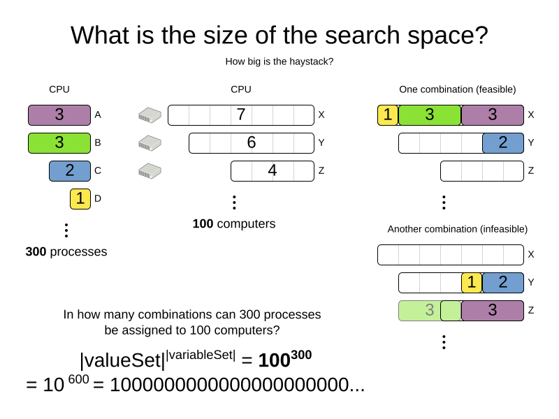
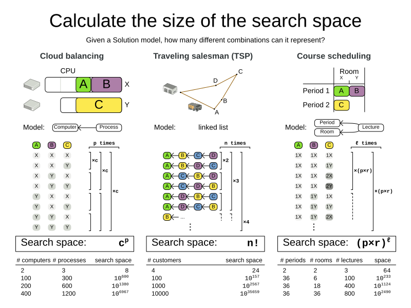
Calculating the number of possible solutions depends on the design of the domain model:
|
This search space size calculation includes infeasible solutions (if they can be represented by the model), because:
Even in cases where adding some of the hard constraints in the formula is practical (for example, Course Scheduling), the resulting search space is still huge. |
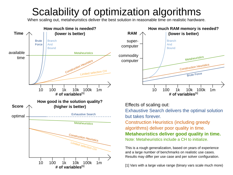
An algorithm that checks every possible solution (even with pruning, such as in Branch And Bound) can easily run for billions of years on a single real-life planning problem. The aim is to find the best solution in the available timeframe. Planning competitions (such as the International Timetabling Competition) show that Local Search variations (Tabu Search, Simulated Annealing, Late Acceptance, …) usually perform best for real-world problems given real-world time limitations.
2. Does OptaPlanner find the optimal solution?
The business wants the optimal solution, but they also have other requirements:
-
Scale out: Large production data sets must not crash and have also good results.
-
Optimize the right problem: The constraints must match the actual business needs.
-
Available time: The solution must be found in time, before it becomes useless to execute.
-
Reliability: Every data set must have at least a decent result (better than a human planner).
Given these requirements, and despite the promises of some salesmen, it is usually impossible for anyone or anything to find the optimal solution. Therefore, OptaPlanner focuses on finding the best solution in available time. In "realistic, independent competitions", it often comes out as the best reusable software.
The nature of NP-complete problems make scaling a prime concern.
|
The quality of a result from a small data set is no indication of the quality of a result from a large data set. |
Scaling issues cannot be mitigated by hardware purchases later on. Start testing with a production sized data set as soon as possible. Do not assess quality on small data sets (unless production encounters only such data sets). Instead, solve a production sized data set and compare the results of longer executions, different algorithms and - if available - the human planner.
3. Architecture overview
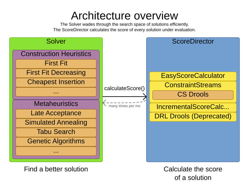
OptaPlanner is the first framework to combine optimization algorithms (metaheuristics, …) with score calculation by a rule engine (such as Drools). This combination is very efficient, because:
-
A rule engine, such as Drools, is great for calculating the score of a solution of a planning problem. It makes it easy and scalable to add additional soft or hard constraints. It does incremental score calculation (deltas) without any extra code. However it tends to be not suitable to actually find new solutions.
-
An optimization algorithm is great at finding new improving solutions for a planning problem, without necessarily brute-forcing every possibility. However, it needs to know the score of a solution and offers no support in calculating that score efficiently.
4. Optimization algorithms overview
OptaPlanner supports three families of optimization algorithms: Exhaustive Search, Construction Heuristics and Metaheuristics. In practice, Metaheuristics (in combination with Construction Heuristics to initialize) are the recommended choice:
Each of these algorithm families have multiple optimization algorithms:
| Algorithm | Scalable? | Optimal? | Easy to use? | Tweakable? | Requires CH? |
|---|---|---|---|---|---|
Exhaustive Search (ES) |
|||||
0/5 |
5/5 |
5/5 |
0/5 |
No |
|
0/5 |
5/5 |
4/5 |
2/5 |
No |
|
Construction heuristics (CH) |
|||||
5/5 |
1/5 |
5/5 |
1/5 |
No |
|
5/5 |
2/5 |
4/5 |
2/5 |
No |
|
5/5 |
2/5 |
4/5 |
2/5 |
No |
|
5/5 |
2/5 |
4/5 |
2/5 |
No |
|
5/5 |
2/5 |
4/5 |
2/5 |
No |
|
5/5 |
2/5 |
4/5 |
2/5 |
No |
|
3/5 |
2/5 |
5/5 |
2/5 |
No |
|
3/5 |
2/5 |
5/5 |
2/5 |
No |
|
Metaheuristics (MH) |
|||||
Local Search (LS) |
|||||
5/5 |
2/5 |
4/5 |
3/5 |
Yes |
|
5/5 |
4/5 |
3/5 |
5/5 |
Yes |
|
5/5 |
4/5 |
2/5 |
5/5 |
Yes |
|
5/5 |
4/5 |
3/5 |
5/5 |
Yes |
|
5/5 |
4/5 |
3/5 |
5/5 |
Yes |
|
5/5 |
4/5 |
3/5 |
5/5 |
Yes |
|
3/5 |
3/5 |
2/5 |
5/5 |
Yes |
|
Evolutionary Algorithms (EA) |
|||||
3/5 |
3/5 |
2/5 |
5/5 |
Yes |
|
3/5 |
3/5 |
2/5 |
5/5 |
Yes |
|
To learn more about metaheuristics, see Essentials of Metaheuristics or Clever Algorithms.
5. Which optimization algorithms should I use?
The best optimization algorithms configuration to use depends heavily on your use case. However, this basic procedure provides a good starting configuration that will produce better than average results.
-
Start with a quick configuration that involves little or no configuration and optimization code: See First Fit.
-
Next, implement planning entity difficulty comparison and turn it into First Fit Decreasing.
-
Next, add Late Acceptance behind it:
-
First Fit Decreasing.
-
At this point, the return on invested time lowers and the result is likely to be sufficient.
However, this can be improved at a lower return on invested time. Use the Benchmarker and try a couple of different Tabu Search, Simulated Annealing and Late Acceptance configurations, for example:
-
First Fit Decreasing: Tabu Search.
Use the Benchmarker to improve the values for the size parameters.
Other experiments can also be run. For example, the following multiple algorithms can be combined together:
-
First Fit Decreasing
-
Late Acceptance (relatively long time)
-
Tabu Search (relatively short time)
6. Power tweaking or default parameter values
Many optimization algorithms have parameters that affect results and scalability. OptaPlanner applies configuration by exception, so all optimization algorithms have default parameter values. This is very similar to the Garbage Collection parameters in a JVM: most users have no need to tweak them, but power users often do.
The default parameter values are sufficient for many cases (and especially for prototypes), but if development time allows, it may be beneficial to power tweak them with the benchmarker for better results and scalability on a specific use case. The documentation for each optimization algorithm also declares the advanced configuration for power tweaking.
|
The default value of parameters will change between minor versions, to improve them for most users. The advanced configuration can be used to prevent unwanted changes, however, this is not recommended. |
7. Solver phase
A Solver can use multiple optimization algorithms in sequence.
Each optimization algorithm is represented by one solver Phase.
There is never more than one Phase solving at the same time.
|
Some |
Here is a configuration that runs three phases in sequence:
<solver xmlns="https://www.optaplanner.org/xsd/solver" xmlns:xsi="http://www.w3.org/2001/XMLSchema-instance"
    xsi:schemaLocation="https://www.optaplanner.org/xsd/solver https://www.optaplanner.org/xsd/solver/solver.xsd">
  ...
  <constructionHeuristic>
    ... <!-- First phase: First Fit Decreasing -->
  </constructionHeuristic>
  <localSearch>
    ... <!-- Second phase: Late Acceptance -->
  </localSearch>
  <localSearch>
    ... <!-- Third phase: Tabu Search -->
  </localSearch>
</solver>
The solver phases are run in the order defined by solver configuration.
-
When the first
Phaseterminates, the secondPhasestarts, and so on. -
When the last
Phaseterminates, theSolverterminates.
Usually, a Solver will first run a construction heuristic and then run one or multiple metaheuristics:
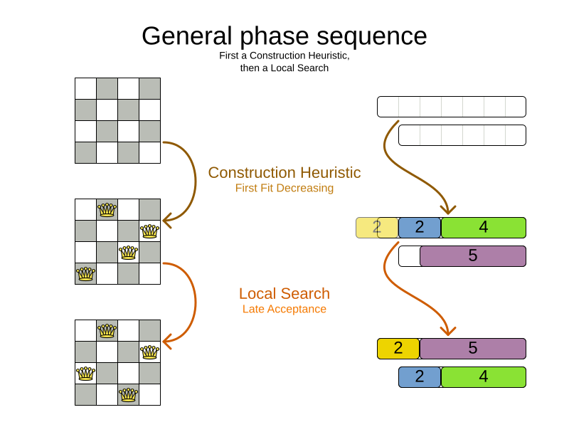
If no phases are configured, OptaPlanner will default to a Construction Heuristic phase followed by a Local Search phase.
Some phases (especially construction heuristics) will terminate automatically.
Other phases (especially metaheuristics) will only terminate if the Phase is configured to terminate:
<solver xmlns="https://www.optaplanner.org/xsd/solver" xmlns:xsi="http://www.w3.org/2001/XMLSchema-instance"
    xsi:schemaLocation="https://www.optaplanner.org/xsd/solver https://www.optaplanner.org/xsd/solver/solver.xsd">
  ...
  <termination><!-- Solver termination -->
    <secondsSpentLimit>90</secondsSpentLimit>
  </termination>
  <localSearch>
    <termination><!-- Phase termination -->
      <secondsSpentLimit>60</secondsSpentLimit><!-- Give the next phase a chance to run too, before the Solver terminates -->
    </termination>
    ...
  </localSearch>
  <localSearch>
    ...
  </localSearch>
</solver>
If the Solver terminates (before the last Phase terminates itself),
the current phase is terminated and all subsequent phases will not run.
8. Scope overview
A solver will iteratively run phases. Each phase will usually iteratively run steps. Each step, in turn, usually iteratively runs moves. These form four nested scopes:
-
Solver
-
Phase
-
Step
-
Move
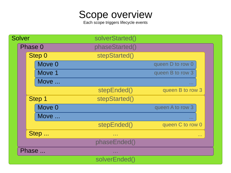
Configure logging to display the log messages of each scope.
9. Termination
Not all phases terminate automatically and may take a significant amount of time.
A Solver can be terminated synchronously by up-front configuration, or asynchronously from another thread.
Metaheuristic phases in particular need to be instructed to stop solving. This can be because of a number of reasons, for example, if the time is up, or the perfect score has been reached just before its solution is used. Finding the optimal solution cannot be relied on (unless you know the optimal score), because a metaheuristic algorithm is generally unaware of the optimal solution.
This is not an issue for real-life problems, as finding the optimal solution may take more time than is available. Finding the best solution in the available time is the most important outcome.
|
If no termination is configured (and a metaheuristic algorithm is used), the |
For synchronous termination, configure a Termination on a Solver or a Phase when it needs to stop.
The built-in implementations of these should be sufficient,
but custom terminations are supported too.
Every Termination can calculate a time gradient (needed for some optimization algorithms),
which is a ratio between the time already spent solving and the estimated entire solving time of the Solver or Phase.
9.1. Time spent termination
Terminates when an amount of time has been used.
  <termination>
    <!-- 2 minutes and 30 seconds in ISO 8601 format P[n]Y[n]M[n]DT[n]H[n]M[n]S -->
    <spentLimit>PT2M30S</spentLimit>
  </termination>
Alternatively to a java.util.Duration in ISO 8601 format, you can also use:
-
Milliseconds
<termination> <millisecondsSpentLimit>500</millisecondsSpentLimit> </termination> -
Seconds
<termination> <secondsSpentLimit>10</secondsSpentLimit> </termination> -
Minutes
<termination> <minutesSpentLimit>5</minutesSpentLimit> </termination> -
Hours
<termination> <hoursSpentLimit>1</hoursSpentLimit> </termination> -
Days
  <termination>
    <daysSpentLimit>2</daysSpentLimit>
  </termination>
Multiple time types can be used together, for example to configure 150 minutes, either configure it directly:
  <termination>
    <minutesSpentLimit>150</minutesSpentLimit>
  </termination>
Or use a combination that sums up to 150 minutes:
  <termination>
    <hoursSpentLimit>2</hoursSpentLimit>
    <minutesSpentLimit>30</minutesSpentLimit>
</termination>|
This
|
9.2. Unimproved time spent termination
Terminates when the best score has not improved in a specified amount of time. Each time a new best solution is found, the timer basically resets.
  <localSearch>
    <termination>
      <!-- 2 minutes and 30 seconds in ISO 8601 format P[n]Y[n]M[n]DT[n]H[n]M[n]S -->
      <unimprovedSpentLimit>PT2M30S</unimprovedSpentLimit>
    </termination>
  </localSearch>
Alternatively to a java.util.Duration in ISO 8601 format, you can also use:
-
Milliseconds
<localSearch> <termination> <unimprovedMillisecondsSpentLimit>500</unimprovedMillisecondsSpentLimit> </termination> </localSearch> -
Seconds
<localSearch> <termination> <unimprovedSecondsSpentLimit>10</unimprovedSecondsSpentLimit> </termination> </localSearch> -
Minutes
<localSearch> <termination> <unimprovedMinutesSpentLimit>5</unimprovedMinutesSpentLimit> </termination> </localSearch> -
Hours
<localSearch> <termination> <unimprovedHoursSpentLimit>1</unimprovedHoursSpentLimit> </termination> </localSearch> -
Days
  <localSearch>
    <termination>
      <unimprovedDaysSpentLimit>1</unimprovedDaysSpentLimit>
    </termination>
  </localSearch>
Just like time spent termination, combinations are summed up.
It is preffered to configure this termination on a specific Phase (such as <localSearch>) instead of on the Solver itself.
|
This
|
Optionally, configure a score difference threshold by which the best score must improve in the specified time.
For example, if the score doesn’t improve by at least 100 soft points every 30 seconds or less, it terminates:
  <localSearch>
    <termination>
      <unimprovedSecondsSpentLimit>30</unimprovedSecondsSpentLimit>
      <unimprovedScoreDifferenceThreshold>0hard/100soft</unimprovedScoreDifferenceThreshold>
    </termination>
  </localSearch>
If the score improves by 1 hard point and drops 900 soft points, it’s still meets the threshold,
because 1hard/-900soft is larger than the threshold 0hard/100soft.
On the other hand, a threshold of 1hard/0soft is not met by any new best solution
that improves 1 hard point at the expense of 1 or more soft points,
because 1hard/-100soft is smaller than the threshold 1hard/0soft.
To require a feasibility improvement every 30 seconds while avoiding the pitfall above,
use a wildcard * for lower score levels that are allowed to deteriorate if a higher score level improves:
  <localSearch>
    <termination>
      <unimprovedSecondsSpentLimit>30</unimprovedSecondsSpentLimit>
      <unimprovedScoreDifferenceThreshold>1hard/*soft</unimprovedScoreDifferenceThreshold>
    </termination>
  </localSearch>
This effectively implies a threshold of 1hard/-2147483648soft, because it relies on Integer.MIN_VALUE.
9.3. BestScoreTermination
BestScoreTermination terminates when a certain score has been reached.
Use this Termination where the perfect score is known, for example for four queens (which uses a SimpleScore):
  <termination>
    <bestScoreLimit>0</bestScoreLimit>
  </termination>
A planning problem with a HardSoftScore may look like this:
  <termination>
    <bestScoreLimit>0hard/-5000soft</bestScoreLimit>
  </termination>
A planning problem with a BendableScore with three hard levels and one soft level may look like this:
  <termination>
    <bestScoreLimit>[0/0/0]hard/[-5000]soft</bestScoreLimit>
  </termination>
In this instance, Termination once a feasible solution has been reached is not practical because it requires a bestScoreLimit such as 0hard/-2147483648soft. Use the next termination instead.
9.4. BestScoreFeasibleTermination
Terminates as soon as a feasible solution has been discovered.
  <termination>
    <bestScoreFeasible>true</bestScoreFeasible>
  </termination>
This Termination is usually combined with other terminations.
9.5. StepCountTermination
Terminates when a number of steps has been reached. This is useful for hardware performance independent runs.
  <localSearch>
    <termination>
      <stepCountLimit>100</stepCountLimit>
    </termination>
  </localSearch>
This Termination can only be used for a Phase (such as <localSearch>), not for the Solver itself.
9.6. UnimprovedStepCountTermination
Terminates when the best score has not improved in a number of steps. This is useful for hardware performance independent runs.
  <localSearch>
    <termination>
      <unimprovedStepCountLimit>100</unimprovedStepCountLimit>
    </termination>
  </localSearch>
If the score has not improved recently, it is unlikely to improve in a reasonable timeframe. It has been observed that once a new best solution is found (even after a long time without improvement on the best solution), the next few steps tend to improve the best solution.
This Termination can only be used for a Phase (such as <localSearch>), not for the Solver itself.
9.7. ScoreCalculationCountTermination
ScoreCalculationCountTermination terminates when a number of score calculations have been reached.
This is often the sum of the number of moves and the number of steps.
This is useful for benchmarking.
  <termination>
    <scoreCalculationCountLimit>100000</scoreCalculationCountLimit>
  </termination>
Switching EnvironmentMode can heavily impact when this termination ends.
9.8. Combining multiple terminations
Terminations can be combined, for example: terminate after 100 steps or if a score of 0 has been reached:
  <termination>
    <terminationCompositionStyle>OR</terminationCompositionStyle>
    <bestScoreLimit>0</bestScoreLimit>
    <stepCountLimit>100</stepCountLimit>
  </termination>
Alternatively you can use AND, for example: terminate after reaching a feasible score of at least -100 and no improvements in 5 steps:
  <termination>
    <terminationCompositionStyle>AND</terminationCompositionStyle>
    <bestScoreLimit>-100</bestScoreLimit>
    <unimprovedStepCountLimit>5</unimprovedStepCountLimit>
  </termination>
This example ensures it does not just terminate after finding a feasible solution, but also completes any obvious improvements on that solution before terminating.
9.9. Asynchronous termination from another thread
Asynchronous termination cannot be configured by a Termination as it is impossible to predict when and if it will occur.
For example, a user action or a server restart could require a solver to terminate earlier than predicted.
To terminate a solver from another thread asynchronously
call the terminateEarly() method from another thread:
solver.terminateEarly();The solver then terminates at its earliest convenience.
After termination, the Solver.solve(Solution) method returns in the solver thread (which is the original thread that called it).
|
When an To guarantee a graceful shutdown of a thread pool that contains solver threads,
an interrupt of a solver thread has the same effect as calling |
10. SolverEventListener
Each time a new best solution is found, a new BestSolutionChangedEvent is fired in the Solver thread.
To listen to such events, add a SolverEventListener to the Solver:
public interface Solver<Solution_> {
    ...

    void addEventListener(SolverEventListener<S> eventListener);
    void removeEventListener(SolverEventListener<S> eventListener);

}
The BestSolutionChangedEvent's newBestSolution may not be initialized or feasible.
Use the isFeasible() method on BestSolutionChangedEvent's new best Score to detect such cases:
    solver.addEventListener(new SolverEventListener<CloudBalance>() {
        public void bestSolutionChanged(BestSolutionChangedEvent<CloudBalance> event) {
            // Ignore infeasible (including uninitialized) solutions
            if (event.getNewBestSolution().getScore().isFeasible()) {
                ...
            }
        }
    });
Use Score.isSolutionInitialized() instead of Score.isFeasible() to only ignore uninitialized solutions, but also accept infeasible solutions.
|
The |
11. Custom solver phase
Run a custom optimization algorithm between phases or before the first phase to initialize the solution, or to get a better score quickly.
You will still want to reuse the score calculation.
For example, to implement a custom Construction Heuristic without implementing an entire Phase.
|
Most of the time, a custom solver phase is not worth the development time investment.
The supported Constructions Heuristics are configurable (use the Benchmarker to tweak them),
|
The CustomPhaseCommand interface appears as follows:
public interface CustomPhaseCommand<Solution_> {
    ...

    void changeWorkingSolution(ScoreDirector<Solution_> scoreDirector);

}
For example, implement CustomPhaseCommand and its changeWorkingSolution() method:
public class ToOriginalMachineSolutionInitializer extends AbstractCustomPhaseCommand<MachineReassignment> {

    public void changeWorkingSolution(ScoreDirector<MachineReassignment> scoreDirector) {
        MachineReassignment machineReassignment = scoreDirector.getWorkingSolution();
        for (MrProcessAssignment processAssignment : machineReassignment.getProcessAssignmentList()) {
            scoreDirector.beforeVariableChanged(processAssignment, "machine");
            processAssignment.setMachine(processAssignment.getOriginalMachine());
            scoreDirector.afterVariableChanged(processAssignment, "machine");
            scoreDirector.triggerVariableListeners();
        }
    }

}|
Any change on the planning entities in a |
|
Do not change any of the problem facts in a |
Configure the CustomPhaseCommand in the solver configuration:
<solver xmlns="https://www.optaplanner.org/xsd/solver" xmlns:xsi="http://www.w3.org/2001/XMLSchema-instance"
    xsi:schemaLocation="https://www.optaplanner.org/xsd/solver https://www.optaplanner.org/xsd/solver/solver.xsd">
  ...
  <customPhase>
    <customPhaseCommandClass>org.optaplanner.examples.machinereassignment.solver.solution.initializer.ToOriginalMachineSolutionInitializer</customPhaseCommandClass>
  </customPhase>
  ... <!-- Other phases -->
</solver>
Configure multiple customPhaseCommandClass instances to run them in sequence.
|
If the changes of a |
|
If the |
To configure values of a CustomPhaseCommand dynamically in the solver configuration
(so the Benchmarker can tweak those parameters),
add the customProperties element and use custom properties:
  <customPhase>
    <customPhaseCommandClass>...MyCustomPhase</customPhaseCommandClass>
    <customProperties>
      <property name="mySelectionSize" value="5"/>
    </customProperties>
  </customPhase>
12. No change solver phase
In rare cases, it’s useful not to run any solver phases.
But by default, configuring no phase will trigger running the default phases.
To avoid those, configure a NoChangePhase:
<solver xmlns="https://www.optaplanner.org/xsd/solver" xmlns:xsi="http://www.w3.org/2001/XMLSchema-instance"
xsi:schemaLocation="https://www.optaplanner.org/xsd/solver https://www.optaplanner.org/xsd/solver/solver.xsd">
...
<noChangePhase/>
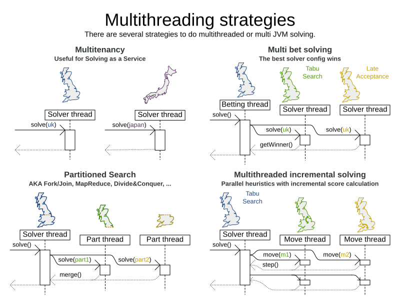
</solver>13. Multithreaded solving
There are several ways of doing multithreaded solving:
-
Multitenancy: solve different datasets in parallel
-
The
SolverManagerwill make it even easier to set this up, in a future version.
-
-
Multi bet solving: solve 1 dataset with multiple, isolated solvers and take the best result.
-
Not recommended: This is a marginal gain for a high cost of hardware resources.
-
Use the Benchmarker during development to determine the most appropriate algorithm, although that’s only on average.
-
Use multithreaded incremental solving instead.
-
-
Partitioned Search: Split 1 dataset in multiple parts and solve them independently.
-
Configure a Partitioned Search.
-
-
Multithreaded incremental solving: solve 1 dataset with multiple threads without sacrificing incremental score calculation.
-
Donate a portion of your CPU cores to OptaPlanner to scale up the score calculation speed and get the same results in fraction of the time.
-
Configure multithreaded incremental solving.
-
|
A logging level of |
13.1. @PlanningId
For some functionality (such as multithreaded solving and real-time planning), OptaPlanner needs to map problem facts and planning entities to an ID. OptaPlanner uses that ID to rebase a move from one thread’s solution state to another’s.
To enable such functionality, specify the @PlanningId annotation on the identification field or getter method,
for example on the database ID:
public class CloudComputer {

    @PlanningId
    private Long id;

    ...
}
Or alternatively, on another type of ID:
public class User {

    @PlanningId
    private String username;

    ...
}
A @PlanningId property must be:
-
Unique for that specific class
-
It does not need to be unique across different problem fact classes (unless in that rare case that those classes are mixed in the same value range or planning entity collection).
-
-
An instance of a type that implements
Object.hashCode()andObject.equals().-
It’s recommended to use the type
Integer,int,Long,long,StringorUUID.
-
-
Never
nullby the timeSolver.solve()is called.
13.2. Custom thread factory (WildFly, Android, GAE, …)
The threadFactoryClass allows to plug in a custom ThreadFactory for environments
where arbitrary thread creation should be avoided,
such as most application servers (including WildFly), Android, or Google App Engine.
Configure the ThreadFactory on the solver to create the move threads
and the Partition Search threads with it:
<solver xmlns="https://www.optaplanner.org/xsd/solver" xmlns:xsi="http://www.w3.org/2001/XMLSchema-instance"
    xsi:schemaLocation="https://www.optaplanner.org/xsd/solver https://www.optaplanner.org/xsd/solver/solver.xsd">
  <threadFactoryClass>...MyAppServerThreadFactory</threadFactoryClass>
  ...
</solver>
13.3. Multithreaded incremental solving
Enable multithreaded incremental solving by adding a @PlanningId annotation
on every planning entity class and planning value class.
Then configure a moveThreadCount:
<solver xmlns="https://www.optaplanner.org/xsd/solver" xmlns:xsi="http://www.w3.org/2001/XMLSchema-instance"
    xsi:schemaLocation="https://www.optaplanner.org/xsd/solver https://www.optaplanner.org/xsd/solver/solver.xsd">
  <moveThreadCount>AUTO</moveThreadCount>
  ...
</solver>
That one extra line heavily improves the score calculation speed, presuming that your machine has enough free CPU cores.
Advanced configuration:
<solver xmlns="https://www.optaplanner.org/xsd/solver" xmlns:xsi="http://www.w3.org/2001/XMLSchema-instance"
    xsi:schemaLocation="https://www.optaplanner.org/xsd/solver https://www.optaplanner.org/xsd/solver/solver.xsd">
  <moveThreadCount>4</moveThreadCount>
  <moveThreadBufferSize>10</moveThreadBufferSize>
  <threadFactoryClass>...MyAppServerThreadFactory</threadFactoryClass>
  ...
</solver>
A moveThreadCount of 4 saturates almost 5 CPU cores:
the 4 move threads fill up 4 CPU cores completely
and the solver thread uses most of another CPU core.
The following moveThreadCounts are supported:
-
NONE(default): Don’t run any move threads. Use the single threaded code. -
AUTO: Let OptaPlanner decide how many move threads to run in parallel. On machines or containers with little or no CPUs, this falls back to the single threaded code. -
Static number: The number of move threads to run in parallel.
<moveThreadCount>4</moveThreadCount>This can be
1to enforce running the multithreaded code with only 1 move thread (which is less efficient thanNONE).
It is counter-effective to set a moveThreadCount
that is higher than the number of available CPU cores,
as that will slow down the score calculation speed.
One good reason to do it anyway, is to reproduce a bug of a high-end production machine.
|
Multithreaded solving is still reproducible, as long as the resolved |
The moveThreadBufferSize power tweaks the number of moves that are selected but won’t be foraged.
Setting it too low reduces performance, but setting it too high too.
Unless you’re deeply familiar with the inner workings of multithreaded solving, don’t configure this parameter.
To run in an environment that doesn’t like arbitrary thread creation,
use threadFactoryClass to plug in a custom thread factory.