Benchmarking and tweaking
1. Find the best solver configuration
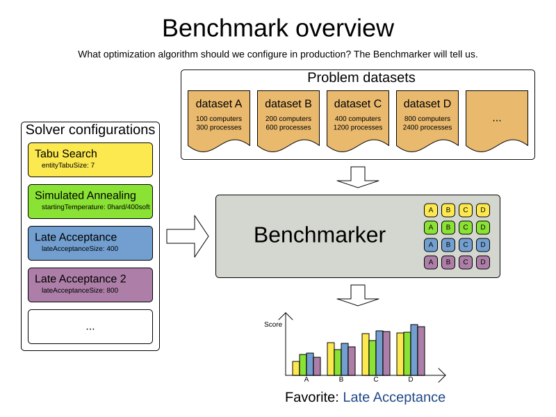
OptaPlanner supports several optimization algorithms, so you’re probably wondering which is the best one? Although some optimization algorithms generally perform better than others, it really depends on your problem domain. Most solver phases have parameters which can be tweaked. Those parameters can influence the results a lot, even though most solver phases work pretty well out-of-the-box.
Luckily, OptaPlanner includes a benchmarker, which allows you to play out different solver phases with different settings against each other in development, so you can use the best configuration for your planning problem in production.
2. Benchmark configuration
2.1. Add a dependency on optaplanner-benchmark
The benchmarker is in a separate artifact called optaplanner-benchmark.
If you use Maven, add a dependency in your pom.xml file:
    <dependency>
      <groupId>org.optaplanner</groupId>
      <artifactId>optaplanner-benchmark</artifactId>
    </dependency>
This is similar for Gradle, Ivy and Buildr.
The version must be exactly the same as the optaplanner-core version used (which is automatically the case if you import optaplanner-bom).
If you use ANT, you’ve probably already copied the required jars from the download zip’s binaries directory.
2.2. Run a simple benchmark
To quickly setup a benchmark, create a PlannerBenchmarkFactory from your solver configuration XML,
load a few datasets and benchmark them. For example, with 3 datasets:
PlannerBenchmarkFactory benchmarkFactory = PlannerBenchmarkFactory.createFromSolverConfigXmlResource(
        "org/optaplanner/examples/cloudbalancing/solver/cloudBalancingSolverConfig.xml");

CloudBalance dataset1 = ...;
CloudBalance dataset2 = ...;
CloudBalance dataset3 = ...;
PlannerBenchmark benchmark = benchmarkFactory.buildPlannerBenchmark(
        dataset1, dataset2, dataset3);
benchmark.benchmarkAndShowReportInBrowser();
This generates a benchmark report in local/benchmarkReport and shows it in your browser when it’s finished.
The SolverFactory's solver configuration needs a termination to limit how long each dataset runs.
To configure a different benchmark directory, pass a File parameter to createFromSolverConfigXmlResource().
The generated benchmark report already contains interesting information, but it doesn’t compare solver configurations to find the best algorithm. To do that, set up an explicit benchmark configuration:
2.3. Configure and run an advanced benchmark
Build a PlannerBenchmark instance with a PlannerBenchmarkFactory.
Configure it with a benchmark configuration XML file, provided as a classpath resource:
PlannerBenchmarkFactory benchmarkFactory = PlannerBenchmarkFactory.createFromXmlResource(
        "org/optaplanner/examples/cloudbalancing/benchmark/cloudBalancingBenchmarkConfig.xml");
PlannerBenchmark benchmark = benchmarkFactory.buildPlannerBenchmark();
benchmark.benchmarkAndShowReportInBrowser();
Alternatively, create a PlannerBenchmarkFactory programmatically from a PlannerBenchmarkConfig.
A benchmark configuration XML file looks like this:
<?xml version="1.0" encoding="UTF-8"?>
<plannerBenchmark xmlns="https://www.optaplanner.org/xsd/benchmark" xmlns:xsi="http://www.w3.org/2001/XMLSchema-instance"
    xsi:schemaLocation="https://www.optaplanner.org/xsd/benchmark https://www.optaplanner.org/xsd/benchmark/benchmark.xsd">
  <benchmarkDirectory>local/data/nqueens</benchmarkDirectory>

  <inheritedSolverBenchmark>
    <solver>
      ...<!-- Common solver configuration -->
    </solver>
    <problemBenchmarks>
      ...
      <inputSolutionFile>data/cloudbalancing/unsolved/100computers-300processes.json</inputSolutionFile>
      <inputSolutionFile>data/cloudbalancing/unsolved/200computers-600processes.json</inputSolutionFile>
    </problemBenchmarks>
  </inheritedSolverBenchmark>

  <solverBenchmark>
    <name>Tabu Search</name>
    <solver>
      ...<!-- Tabu Search specific solver configuration -->
    </solver>
  </solverBenchmark>
  <solverBenchmark>
    <name>Simulated Annealing</name>
    <solver>
      ...<!-- Simulated Annealing specific solver configuration -->
    </solver>
  </solverBenchmark>
  <solverBenchmark>
    <name>Late Acceptance</name>
    <solver>
      ...<!-- Late Acceptance specific solver configuration -->
    </solver>
  </solverBenchmark>
</plannerBenchmark>
This PlannerBenchmark tries three configurations (Tabu Search, Simulated Annealing and Late Acceptance)
on two data sets (100computers-300processes and 200computers-600processes), so it runs six solvers.
Every <solverBenchmark> element contains a solver configuration and one or more <inputSolutionFile> elements.
It runs the solver configuration on each of those unsolved solution files.
The element name is optional, because it is generated if absent.
The inputSolutionFile is read by a SolutionFileIO, relative to the working directory.
|
Use a forward slash ( Do not use backslash ( |
The benchmark report is written in the directory specified by the <benchmarkDirectory> element (relative to the working directory).
|
It’s recommended that the |
If an Exception or Error occurs in a single benchmark, the entire Benchmarker does not fail-fast (unlike everything else in OptaPlanner).
Instead, the Benchmarker continues to run all other benchmarks, write the benchmark report and then fail (if there is at least one failing single benchmark).
The failing benchmarks are clearly marked as such in the benchmark report.
2.3.1. Inherited solver benchmark
To lower verbosity, the common parts of multiple <solverBenchmark> elements are extracted to the <inheritedSolverBenchmark> element.
Every property can still be overwritten per <solverBenchmark> element.
Note that inherited solver phases such as <constructionHeuristic> or <localSearch> are not overwritten
but instead are added to the tail of the solver phases list.
2.4. SolutionFileIO: input and output of solution files
2.4.1. SolutionFileIO interface
The benchmarker needs to be able to read the input files to load a problem.
Also, it optionally writes the best solution of each benchmark to an output file.
It does that through the SolutionFileIO interface which has a read and write method:
public interface SolutionFileIO<Solution_> {
    ...

    Solution_ read(File inputSolutionFile);
    void write(Solution_ solution, File outputSolutionFile);

}
The SolutionFileIO interface is in the optaplanner-persistence-common jar (which is a dependency of the optaplanner-benchmark jar).
There are several ways to serialize a solution.
2.4.2. JacksonSolutionFileIO: serialize to and from an JSON format
To read and write solutions in JSON format via Jackson, extend the JacksonSolutionFileIO:
public class NQueensJsonSolutionFileIO extends JacksonSolutionFileIO<NQueens> {
    public NQueensJsonSolutionFileIO() {
        // NQueens is the @PlanningSolution class.
        super(NQueens.class);
    }
}
If the JSON file requires specific Jackson modules and features to be enabled/disabled. You could create your desired object mapper as a dependency to the JacksonSolutionFileIO as follows:
public class NQueensJsonSolutionFileIO extends JacksonSolutionFileIO<NQueens> {
    public NQueensJsonSolutionFileIO() {
        // NQueens is the @PlanningSolution class.
        super(NQueens.class,
                new ObjectMapper()
                        .registerModule(new JavaTimeModule())
                        .disable(SerializationFeature.WRITE_DATES_AS_TIMESTAMPS)
        );
    }

}
Then use it in the benchmark configuration like so:
    <problemBenchmarks>
      <solutionFileIOClass>org.optaplanner.examples.nqueens.persistence.NQueensJsonSolutionFileIO</solutionFileIOClass>
      <inputSolutionFile>data/nqueens/unsolved/32queens.json</inputSolutionFile>
      ...
    </problemBenchmarks>
2.4.3. JaxbSolutionFileIO: serialize to and from an XML format
To read and write solutions in the XML format via Java Architecture for XML Binding (JAXB), extend the JaxbSolutionFileIO:
public class NQueensXmlSolutionFileIO extends JaxbSolutionFileIO<NQueens> {
    public NQueensXmlSolutionFileIO() {
        // NQueens is the @PlanningSolution class.
        super(NQueens.class);
    }
}
and use it in the benchmark configuration:
    <problemBenchmarks>
      <solutionFileIOClass>org.optaplanner.examples.nqueens.persistence.NQueensSolutionFileIO</solutionFileIOClass>
      <inputSolutionFile>data/nqueens/unsolved/32queens.xml</inputSolutionFile>
      ...
    </problemBenchmarks>
Add JAXB annotations (such as @XmlElement) on your domain classes to use a less verbose XML format.
Regardless, XML is still a very verbose format.
Reading or writing large datasets in this format can cause an OutOfMemoryError, StackOverflowError
or large performance degradation.
2.4.4. Custom SolutionFileIO: serialize to and from a custom format
Implement your own SolutionFileIO implementation and configure it with the solutionFileIOClass element to write to a custom format (such as a txt or a binary format):
    <problemBenchmarks>
      <solutionFileIOClass>org.optaplanner.examples.machinereassignment.persistence.MachineReassignmentFileIO</solutionFileIOClass>
      <inputSolutionFile>data/machinereassignment/import/model_a1_1.txt</inputSolutionFile>
      ...
    </problemBenchmarks>
It’s recommended that output files can be read as input files,
which implies that getInputFileExtension() and getOutputFileExtension() return the same value.
|
A |
2.4.5. Reading an input solution from a database or other storage
There are two options if your dataset is in a relational database or another type of repository:
-
Extract the datasets from the database and serialize them to a local file, for example as JSON with
JacksonSolutionFileIO. Then use those files in<inputSolutionFile>elements.-
The benchmarks are now more reliable because they run offline.
-
Each dataset is only loaded just in time.
-
-
Load all the datasets in advance and pass them to the
buildPlannerBenchmark()method:PlannerBenchmark plannerBenchmark = benchmarkFactory.buildPlannerBenchmark(dataset1, dataset2, dataset3);
2.5. Warming up the HotSpot compiler
Without a warm up, the results of the first (or first few) benchmarks are not reliable because they lose CPU time on HotSpot JIT compilation.
To avoid that distortion, the benchmarker runs some of the benchmarks for 30 seconds, before running the real benchmarks. That default warm up of 30 seconds usually suffices. Change it, for example to give it 60 seconds:
<plannerBenchmark xmlns="https://www.optaplanner.org/xsd/benchmark" xmlns:xsi="http://www.w3.org/2001/XMLSchema-instance"
    xsi:schemaLocation="https://www.optaplanner.org/xsd/benchmark https://www.optaplanner.org/xsd/benchmark/benchmark.xsd">
  ...
  <warmUpSecondsSpentLimit>60</warmUpSecondsSpentLimit>
  ...
</plannerBenchmark>
Turn off the warm up phase altogether by setting it to zero:
<plannerBenchmark xmlns="https://www.optaplanner.org/xsd/benchmark" xmlns:xsi="http://www.w3.org/2001/XMLSchema-instance"
    xsi:schemaLocation="https://www.optaplanner.org/xsd/benchmark https://www.optaplanner.org/xsd/benchmark/benchmark.xsd">
  ...
  <warmUpSecondsSpentLimit>0</warmUpSecondsSpentLimit>
  ...
</plannerBenchmark>|
The warm up time budget does not include the time it takes to load the datasets. With large datasets, this can cause the warm up to run considerably longer than specified in the configuration. |
2.6. Benchmark blueprint: a predefined configuration
To quickly configure and run a benchmark for typical solver configs, use a solverBenchmarkBluePrint instead of solverBenchmarks:
<?xml version="1.0" encoding="UTF-8"?>
<plannerBenchmark xmlns="https://www.optaplanner.org/xsd/benchmark" xmlns:xsi="http://www.w3.org/2001/XMLSchema-instance"
    xsi:schemaLocation="https://www.optaplanner.org/xsd/benchmark https://www.optaplanner.org/xsd/benchmark/benchmark.xsd">
  <benchmarkDirectory>local/data/nqueens</benchmarkDirectory>

  <inheritedSolverBenchmark>
    <solver>
      <solutionClass>org.optaplanner.examples.nqueens.domain.NQueens</solutionClass>
      <entityClass>org.optaplanner.examples.nqueens.domain.Queen</entityClass>
      <scoreDirectorFactory>
        <constraintProviderClass>org.optaplanner.examples.nqueens.score.NQueensConstraintProvider</constraintProviderClass>
        <initializingScoreTrend>ONLY_DOWN</initializingScoreTrend>
      </scoreDirectorFactory>
      <termination>
        <minutesSpentLimit>1</minutesSpentLimit>
      </termination>
    </solver>
    <problemBenchmarks>
      <solutionFileIOClass>org.optaplanner.examples.nqueens.persistence.NQueensSolutionFileIO</solutionFileIOClass>
      <inputSolutionFile>data/nqueens/unsolved/32queens.json</inputSolutionFile>
      <inputSolutionFile>data/nqueens/unsolved/64queens.json</inputSolutionFile>
    </problemBenchmarks>
  </inheritedSolverBenchmark>

  <solverBenchmarkBluePrint>
    <solverBenchmarkBluePrintType>EVERY_CONSTRUCTION_HEURISTIC_TYPE_WITH_EVERY_LOCAL_SEARCH_TYPE</solverBenchmarkBluePrintType>
  </solverBenchmarkBluePrint>
</plannerBenchmark>
The following SolverBenchmarkBluePrintTypes are supported:
-
CONSTRUCTION_HEURISTIC_WITH_AND_WITHOUT_LOCAL_SEARCH: Run the default Construction Heuristic type with and without the default Local Search type. -
EVERY_CONSTRUCTION_HEURISTIC_TYPE: Run every Construction Heuristic type (First Fit, First Fit Decreasing, Cheapest Insertion, …). -
EVERY_LOCAL_SEARCH_TYPE: Run every Local Search type (Tabu Search, Late Acceptance, …) with the default Construction Heuristic. -
EVERY_CONSTRUCTION_HEURISTIC_TYPE_WITH_EVERY_LOCAL_SEARCH_TYPE: Run every Construction Heuristic type with every Local Search type.
2.7. Write the output solution of benchmark runs
The best solution of each benchmark run can be written in the benchmarkDirectory.
By default, this is disabled, because the files are rarely used and considered bloat.
Also, on large datasets, writing the best solution of each single benchmark can take quite some time and memory (causing an OutOfMemoryError), especially in a verbose format like XML.
To write those solutions in the benchmarkDirectory, enable writeOutputSolutionEnabled:
    <problemBenchmarks>
      ...
      <writeOutputSolutionEnabled>true</writeOutputSolutionEnabled>
      ...
    </problemBenchmarks>
2.8. Benchmark logging
Benchmark logging is configured like solver logging.
To separate the log messages of each single benchmark run into a separate file, use the MDC with key subSingleBenchmark.name in a sifting appender.
For example with Logback in logback.xml:
  <appender name="fileAppender" class="ch.qos.logback.classic.sift.SiftingAppender">
    <discriminator>
      <key>subSingleBenchmark.name</key>
      <defaultValue>app</defaultValue>
    </discriminator>
    <sift>
      <appender name="fileAppender.${subSingleBenchmark.name}" class="...FileAppender">
        <file>local/log/optaplannerBenchmark-${subSingleBenchmark.name}.log</file>
        ...
      </appender>
    </sift>
  </appender>
3. Benchmark report
3.1. HTML report
After running a benchmark, an HTML report will be written in the benchmarkDirectory with the index.html filename.
Open it in your browser.
It has a nice overview of your benchmark including:
-
Summary statistics: graphs and tables
-
Problem statistics per
inputSolutionFile: graphs and CSV -
Each solver configuration (ranked): Handy to copy and paste
-
Benchmark information: settings, hardware, …
|
Graphs are generated by the excellent JFreeChart library. |
The HTML report will use your default locale to format numbers.
If you share the benchmark report with people from another country, consider overwriting the locale accordingly:
<plannerBenchmark xmlns="https://www.optaplanner.org/xsd/benchmark" xmlns:xsi="http://www.w3.org/2001/XMLSchema-instance"
    xsi:schemaLocation="https://www.optaplanner.org/xsd/benchmark https://www.optaplanner.org/xsd/benchmark/benchmark.xsd">
  ...
  <benchmarkReport>
    <locale>en_US</locale>
  </benchmarkReport>
  ...
</plannerBenchmark>
3.2. Ranking the solvers
The benchmark report automatically ranks the solvers.
The Solver with rank 0 is called the favorite Solver: it performs best overall, but it might not be the best on every problem.
It’s recommended to use that favorite Solver in production.
However, there are different ways of ranking the solvers. Configure it like this:
<plannerBenchmark xmlns="https://www.optaplanner.org/xsd/benchmark" xmlns:xsi="http://www.w3.org/2001/XMLSchema-instance"
    xsi:schemaLocation="https://www.optaplanner.org/xsd/benchmark https://www.optaplanner.org/xsd/benchmark/benchmark.xsd">
  ...
  <benchmarkReport>
    <solverRankingType>TOTAL_SCORE</solverRankingType>
  </benchmarkReport>
  ...
</plannerBenchmark>
The following solverRankingTypes are supported:
-
TOTAL_SCORE(default): Maximize the overall score, so minimize the overall cost if all solutions would be executed. -
WORST_SCORE: Minimize the worst case scenario. -
TOTAL_RANKING: Maximize the overall ranking. Use this if your datasets differ greatly in size or difficulty, producing a difference inScoremagnitude.
Solvers with at least one failed single benchmark do not get a ranking.
Solvers with not fully initialized solutions are ranked worse.
To use a custom ranking, implement a Comparator:
  <benchmarkReport>
    <solverRankingComparatorClass>...TotalScoreSolverRankingComparator</solverRankingComparatorClass>
  </benchmarkReport>
Or by implementing a weight factory:
  <benchmarkReport>
    <solverRankingWeightFactoryClass>...TotalRankSolverRankingWeightFactory</solverRankingWeightFactoryClass>
  </benchmarkReport>
4. Summary statistics
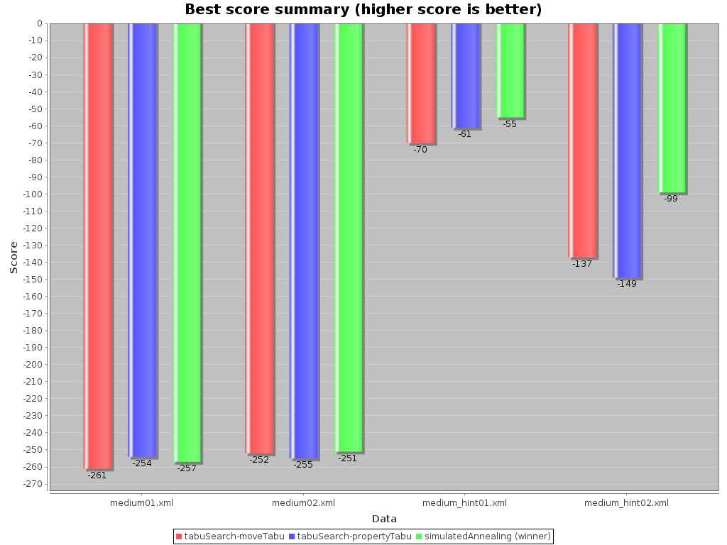
4.1. Best score summary (graph and table)
Shows the best score per inputSolutionFile for each solver configuration.
Useful for visualizing the best solver configuration.
4.2. Best score scalability summary (graph)
Shows the best score per problem scale for each solver configuration.
Useful for visualizing the scalability of each solver configuration.
|
The problem scale will report |
4.3. Best score distribution summary (graph)
Shows the best score distribution per inputSolutionFile for each solver configuration.
Useful for visualizing the reliability of each solver configuration.
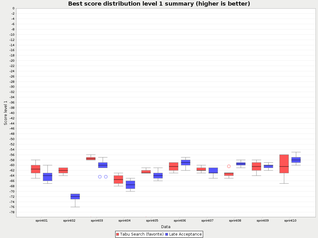
Enable statistical benchmarking to use this summary.
4.4. Winning score difference summary (graph And table)
Shows the winning score difference per inputSolutionFile for each solver configuration.
The winning score difference is the score difference with the score of the winning solver configuration for that particular inputSolutionFile.
Useful for zooming in on the results of the best score summary.
4.5. Worst score difference percentage (ROI) summary (graph And table)
Shows the return on investment (ROI) per inputSolutionFile for each solver configuration if you’d upgrade from the worst solver configuration for that particular inputSolutionFile.
Useful for visualizing the return on investment (ROI) to decision makers.
4.6. Score calculation speed summary (graph And table)
Shows the score calculation speed: a count per second per problem scale for each solver configuration.
Useful for comparing different score calculators and/or constraint implementations (presuming that the solver configurations do not differ otherwise). Also useful to measure the scalability cost of an extra constraint.
4.7. Time spent summary (graph And table)
Shows the time spent per inputSolutionFile for each solver configuration.
This is pointless if it’s benchmarking against a fixed time limit.
Useful for visualizing the performance of construction heuristics (presuming that no other solver phases are configured).
4.8. Time spent scalability summary (graph)
Shows the time spent per problem scale for each solver configuration. This is pointless if it’s benchmarking against a fixed time limit.
Useful for extrapolating the scalability of construction heuristics (presuming that no other solver phases are configured).
4.9. Best score per time spent summary (graph)
Shows the best score per time spent for each solver configuration. This is pointless if it’s benchmarking against a fixed time limit.
Useful for visualizing trade-off between the best score versus the time spent for construction heuristics (presuming that no other solver phases are configured).
5. Statistic per dataset (graph and CSV)
5.1. Enable a problem statistic
The benchmarker supports outputting problem statistics as graphs and CSV (comma separated values) files to the benchmarkDirectory.
To configure one or more, add a problemStatisticType line for each one:
<plannerBenchmark xmlns="https://www.optaplanner.org/xsd/benchmark" xmlns:xsi="http://www.w3.org/2001/XMLSchema-instance"
    xsi:schemaLocation="https://www.optaplanner.org/xsd/benchmark https://www.optaplanner.org/xsd/benchmark/benchmark.xsd">
  <benchmarkDirectory>local/data/nqueens/solved</benchmarkDirectory>
  <inheritedSolverBenchmark>
    <problemBenchmarks>
      ...
      <problemStatisticType>BEST_SCORE</problemStatisticType>
      <problemStatisticType>SCORE_CALCULATION_SPEED</problemStatisticType>
    </problemBenchmarks>
    ...
  </inheritedSolverBenchmark>
  ...
</plannerBenchmark>|
These problem statistics can slow down the solvers noticeably, which affects the benchmark results.
That’s why they are optional and only The summary statistics do not slow down the solver and are always generated. |
The following types are supported:
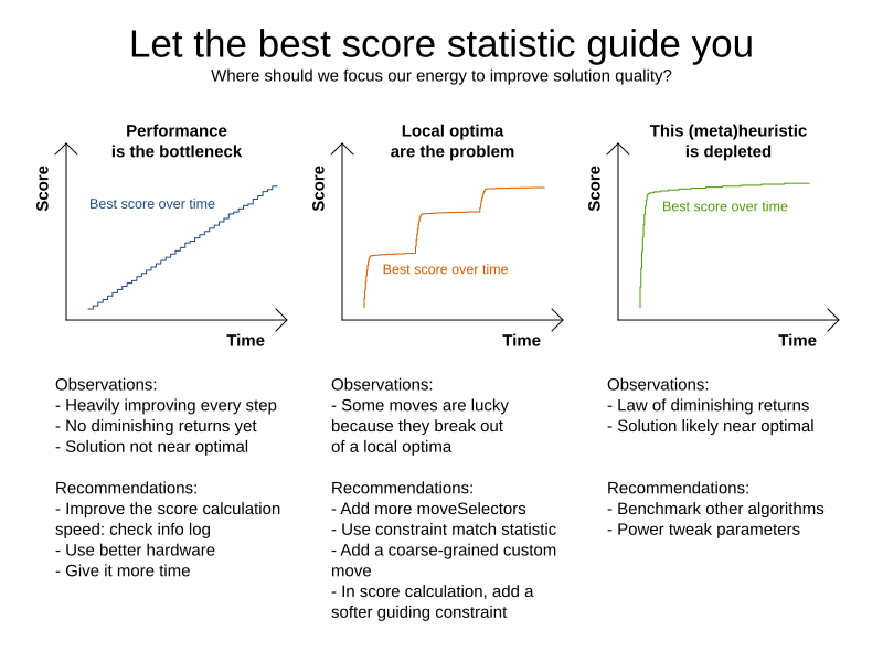
5.2. Best score over time statistic (graph and CSV)
Shows how the best score evolves over time. It is run by default. To run it when other statistics are configured, also add:
    <problemBenchmarks>
      ...
      <problemStatisticType>BEST_SCORE</problemStatisticType>
    </problemBenchmarks>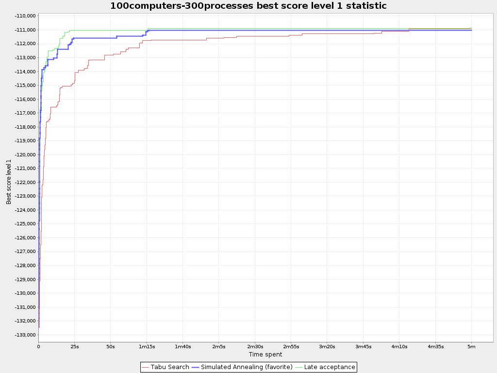
|
A time gradient based algorithm (such as Simulated Annealing) will have a different statistic if it’s run with a different time limit configuration. That’s because this Simulated Annealing implementation automatically determines its velocity based on the amount of time that can be spent. On the other hand, for the Tabu Search and Late Acceptance, what you see is what you’d get. |
The best score over time statistic is very useful to detect abnormalities, such as a potential score trap which gets the solver temporarily stuck in a local optima.
5.3. Step score over time statistic (graph and CSV)
To see how the step score evolves over time, add:
    <problemBenchmarks>
      ...
      <problemStatisticType>STEP_SCORE</problemStatisticType>
    </problemBenchmarks>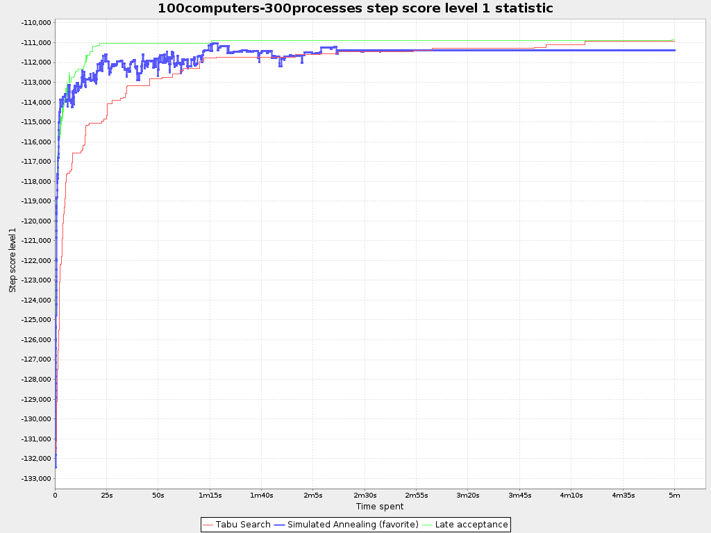
Compare the step score statistic with the best score statistic (especially on parts for which the best score flatlines). If it hits a local optima, the solver should take deteriorating steps to escape it. But it shouldn’t deteriorate too much either.
|
The step score statistic has been seen to slow down the solver noticeably due to GC stress, especially for fast stepping algorithms (such as Simulated Annealing and Late Acceptance). |
5.4. Score calculation speed over time statistic (graph and CSV)
To see how fast the scores are calculated, add:
    <problemBenchmarks>
      ...
      <problemStatisticType>SCORE_CALCULATION_SPEED</problemStatisticType>
    </problemBenchmarks>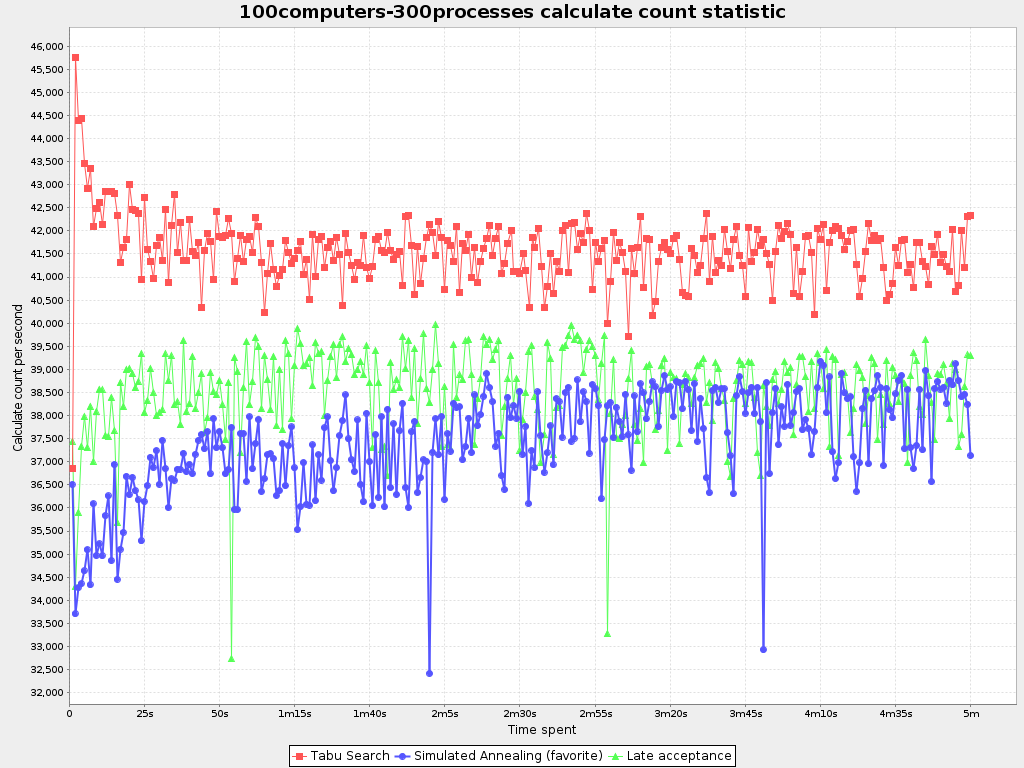
|
The initial high calculation speed is typical during solution initialization: it’s far easier to calculate the score of a solution if only a handful planning entities have been initialized, than when all the planning entities are initialized. After those few seconds of initialization, the calculation speed is relatively stable, apart from an occasional stop-the-world garbage collector disruption. |
5.5. Best solution mutation over time statistic (graph and CSV)
To see how much each new best solution differs from the previous best solution, by counting the number of planning variables which have a different value (not including the variables that have changed multiple times but still end up with the same value), add:
    <problemBenchmarks>
      ...
      <problemStatisticType>BEST_SOLUTION_MUTATION</problemStatisticType>
    </problemBenchmarks>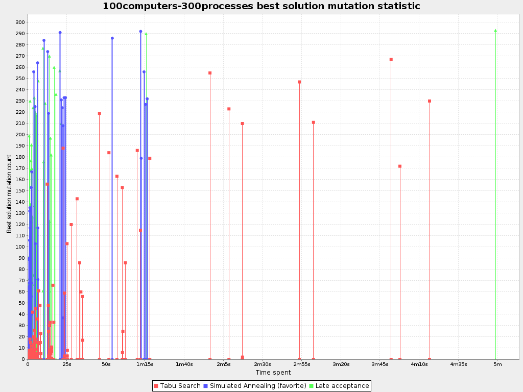
Use Tabu Search - an algorithm that behaves like a human - to get an estimation on how difficult it would be for a human to improve the previous best solution to that new best solution.
5.6. Move count per step statistic (graph and CSV)
To see how the selected and accepted move count per step evolves over time, add:
    <problemBenchmarks>
      ...
      <problemStatisticType>MOVE_COUNT_PER_STEP</problemStatisticType>
    </problemBenchmarks>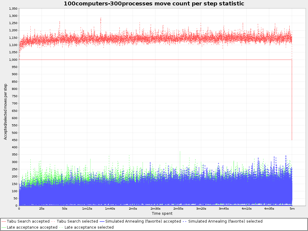
|
This statistic has been seen to slow down the solver noticeably due to GC stress, especially for fast stepping algorithms (such as Simulated Annealing and Late Acceptance). |
6. Statistic per single benchmark (graph and CSV)
6.1. Enable a single statistic
A single statistic is static for one dataset for one solver configuration. Unlike a problem statistic, it does not aggregate over solver configurations.
The benchmarker supports outputting single statistics as graphs and CSV (comma separated values) files to the benchmarkDirectory.
To configure one, add a singleStatisticType line:
<plannerBenchmark xmlns="https://www.optaplanner.org/xsd/benchmark" xmlns:xsi="http://www.w3.org/2001/XMLSchema-instance"
    xsi:schemaLocation="https://www.optaplanner.org/xsd/benchmark https://www.optaplanner.org/xsd/benchmark/benchmark.xsd">
  <benchmarkDirectory>local/data/nqueens/solved</benchmarkDirectory>
  <inheritedSolverBenchmark>
    <problemBenchmarks>
      ...
      <problemStatisticType>...</problemStatisticType>
      <singleStatisticType>PICKED_MOVE_TYPE_BEST_SCORE_DIFF</singleStatisticType>
    </problemBenchmarks>
    ...
  </inheritedSolverBenchmark>
  ...
</plannerBenchmark>
Multiple singleStatisticType elements are allowed.
|
These statistic per single benchmark can slow down the solver noticeably, which affects the benchmark results. That’s why they are optional and not enabled by default. |
The following types are supported:
6.2. Constraint match total best score over time statistic (graph and CSV)
To see which constraints are matched in the best score (and how much) over time, add:
    <problemBenchmarks>
      ...
      <singleStatisticType>CONSTRAINT_MATCH_TOTAL_BEST_SCORE</singleStatisticType>
    </problemBenchmarks>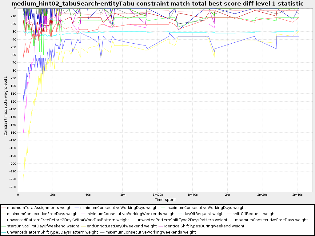
Requires the score calculation to support constraint matches. Constraint Streams and Drools score calculation (Deprecated) support constraint matches automatically, but incremental Java score calculation requires more work.
|
The constraint match total statistics affect the solver noticeably. |
6.3. Constraint match total step score over time statistic (graph and CSV)
To see which constraints are matched in the step score (and how much) over time, add:
    <problemBenchmarks>
      ...
      <singleStatisticType>CONSTRAINT_MATCH_TOTAL_STEP_SCORE</singleStatisticType>
    </problemBenchmarks>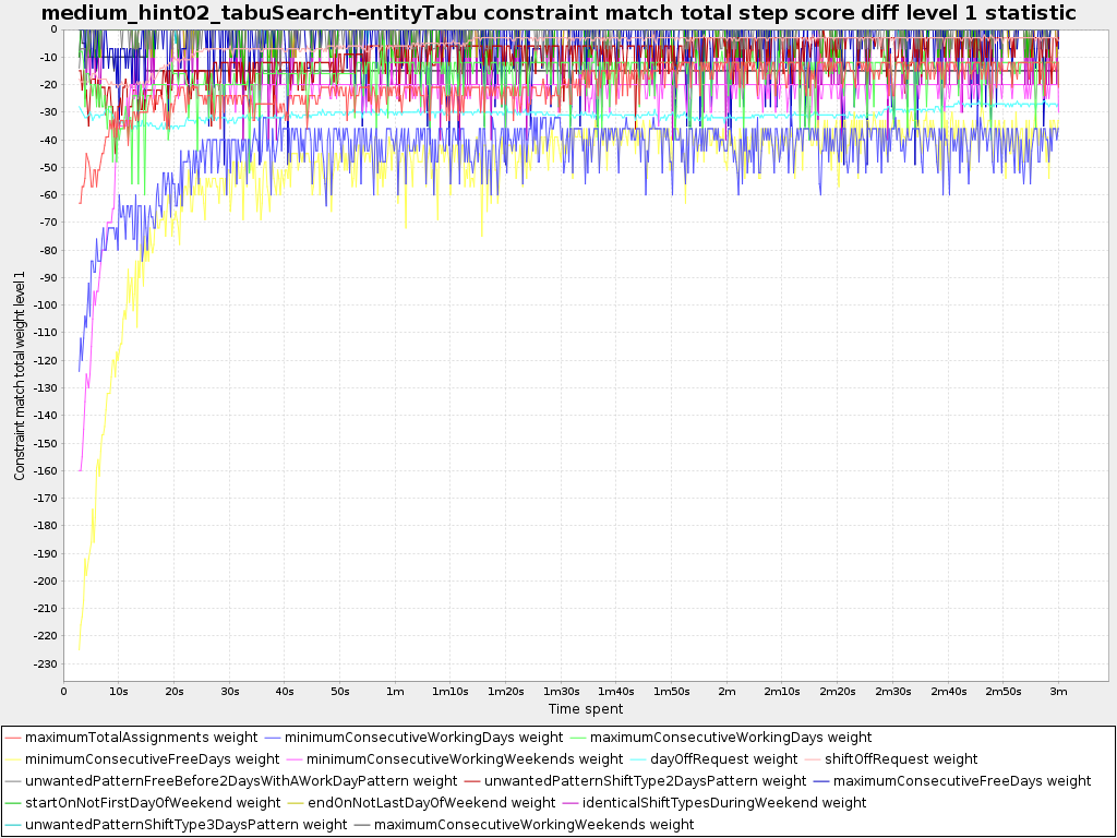
Also requires the score calculation to support constraint matches.
|
The constraint match total statistics affect the solver noticeably. |
6.4. Picked move type best score diff over time statistic (graph and CSV)
To see which move types improve the best score (and how much) over time, add:
    <problemBenchmarks>
      ...
      <singleStatisticType>PICKED_MOVE_TYPE_BEST_SCORE_DIFF</singleStatisticType>
    </problemBenchmarks>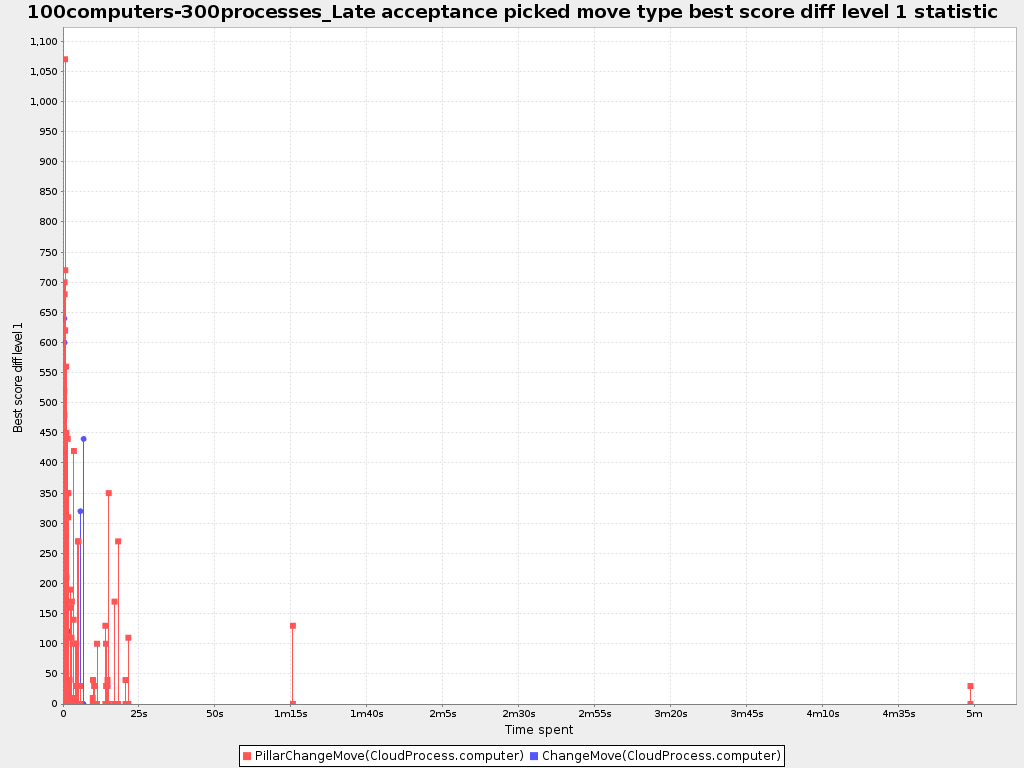
6.5. Picked move type step score diff over time statistic (graph and CSV)
To see how much each winning step affects the step score over time, add:
    <problemBenchmarks>
      ...
      <singleStatisticType>PICKED_MOVE_TYPE_STEP_SCORE_DIFF</singleStatisticType>
    </problemBenchmarks>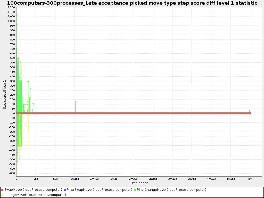
7. Advanced benchmarking
7.1. Benchmarking performance tricks
7.1.1. Parallel benchmarking on multiple threads
If you have multiple processors available on your computer, you can run multiple benchmarks in parallel on multiple threads to get your benchmarks results faster:
<plannerBenchmark xmlns="https://www.optaplanner.org/xsd/benchmark" xmlns:xsi="http://www.w3.org/2001/XMLSchema-instance"
    xsi:schemaLocation="https://www.optaplanner.org/xsd/benchmark https://www.optaplanner.org/xsd/benchmark/benchmark.xsd">
  ...
  <parallelBenchmarkCount>AUTO</parallelBenchmarkCount>
  ...
</plannerBenchmark>|
Running too many benchmarks in parallel will affect the results of benchmarks negatively. Leave some processors unused for garbage collection and other processes. |
The following parallelBenchmarkCounts are supported:
-
1(default): Run all benchmarks sequentially. -
AUTO: Let OptaPlanner decide how many benchmarks to run in parallel. This formula is based on experience. It’s recommended to prefer this over the other parallel enabling options. -
Static number: The number of benchmarks to run in parallel.
<parallelBenchmarkCount>2</parallelBenchmarkCount>
|
The |
|
If you have a computer with slow or unreliable cooling, increasing the The |
The benchmarker uses a thread pool internally, but you can optionally plug in a custom ThreadFactory,
for example when running benchmarks on an application server or a cloud platform:
<plannerBenchmark xmlns="https://www.optaplanner.org/xsd/benchmark" xmlns:xsi="http://www.w3.org/2001/XMLSchema-instance"
    xsi:schemaLocation="https://www.optaplanner.org/xsd/benchmark https://www.optaplanner.org/xsd/benchmark/benchmark.xsd">
  ...
  <threadFactoryClass>...MyCustomThreadFactory</threadFactoryClass>
  ...
</plannerBenchmark>|
In the future, we will also support multi-JVM benchmarking. This feature is independent of multithreaded solving or multi-JVM solving. |
7.2. Statistical benchmarking
To minimize the influence of your environment and the Random Number Generator on the benchmark results, configure the number of times each single benchmark run is repeated. The results of those runs are statistically aggregated. Each individual result is also visible in the report, as well as plotted in the best score distribution summary.
Just add a <subSingleCount> element to an <inheritedSolverBenchmark> element or in a <solverBenchmark> element:
<?xml version="1.0" encoding="UTF-8"?>
<plannerBenchmark xmlns="https://www.optaplanner.org/xsd/benchmark" xmlns:xsi="http://www.w3.org/2001/XMLSchema-instance"
    xsi:schemaLocation="https://www.optaplanner.org/xsd/benchmark https://www.optaplanner.org/xsd/benchmark/benchmark.xsd">
  ...
  <inheritedSolverBenchmark>
    ...
    <solver>
      ...
    </solver>
    <subSingleCount>10</subSingleCount>
  </inheritedSolverBenchmark>
  ...
</plannerBenchmark>
The subSingleCount defaults to 1 (so no statistical benchmarking).
|
If |
7.3. Template-based benchmarking and matrix benchmarking
Matrix benchmarking is benchmarking a combination of value sets.
For example: benchmark four entityTabuSize values (5, 7, 11 and 13) combined with three acceptedCountLimit values (500, 1000 and 2000), resulting in 12 solver configurations.
To reduce the verbosity of such a benchmark configuration, you can use a Freemarker template for the benchmark configuration instead:
<plannerBenchmark xmlns="https://www.optaplanner.org/xsd/benchmark" xmlns:xsi="http://www.w3.org/2001/XMLSchema-instance"
    xsi:schemaLocation="https://www.optaplanner.org/xsd/benchmark https://www.optaplanner.org/xsd/benchmark/benchmark.xsd">
  ...
  <inheritedSolverBenchmark>
    ...
  </inheritedSolverBenchmark>

<#list [5, 7, 11, 13] as entityTabuSize>
<#list [500, 1000, 2000] as acceptedCountLimit>
  <solverBenchmark>
    <name>Tabu Search entityTabuSize ${entityTabuSize} acceptedCountLimit ${acceptedCountLimit}</name>
    <solver>
      <localSearch>
        <unionMoveSelector>
          <changeMoveSelector/>
          <swapMoveSelector/>
        </unionMoveSelector>
        <acceptor>
          <entityTabuSize>${entityTabuSize}</entityTabuSize>
        </acceptor>
        <forager>
          <acceptedCountLimit>${acceptedCountLimit}</acceptedCountLimit>
        </forager>
      </localSearch>
    </solver>
  </solverBenchmark>
</#list>
</#list>
</plannerBenchmark>
To configure Matrix Benchmarking for Simulated Annealing (or any other configuration that involves a Score template variable), use the replace() method in the solver benchmark name element:
<plannerBenchmark xmlns="https://www.optaplanner.org/xsd/benchmark" xmlns:xsi="http://www.w3.org/2001/XMLSchema-instance"
    xsi:schemaLocation="https://www.optaplanner.org/xsd/benchmark https://www.optaplanner.org/xsd/benchmark/benchmark.xsd">
  ...
  <inheritedSolverBenchmark>
    ...
  </inheritedSolverBenchmark>

<#list ["1hard/10soft", "1hard/20soft", "1hard/50soft", "1hard/70soft"] as startingTemperature>
  <solverBenchmark>
    <name>Simulated Annealing startingTemperature ${startingTemperature?replace("/", "_")}</name>
    <solver>
      <localSearch>
        <acceptor>
          <simulatedAnnealingStartingTemperature>${startingTemperature}</simulatedAnnealingStartingTemperature>
        </acceptor>
      </localSearch>
    </solver>
  </solverBenchmark>
</#list>
</plannerBenchmark>|
A solver benchmark name doesn’t allow some characters (such a |
And build it with the class PlannerBenchmarkFactory:
        PlannerBenchmarkFactory benchmarkFactory = PlannerBenchmarkFactory.createFromFreemarkerXmlResource(
                "org/optaplanner/examples/cloudbalancing/optional/benchmark/cloudBalancingBenchmarkConfigTemplate.xml.ftl");
        PlannerBenchmark benchmark = benchmarkFactory.buildPlannerBenchmark();
7.4. Benchmark report aggregation
The BenchmarkAggregator takes one or more existing benchmarks and merges them into new benchmark report, without actually running the benchmarks again.
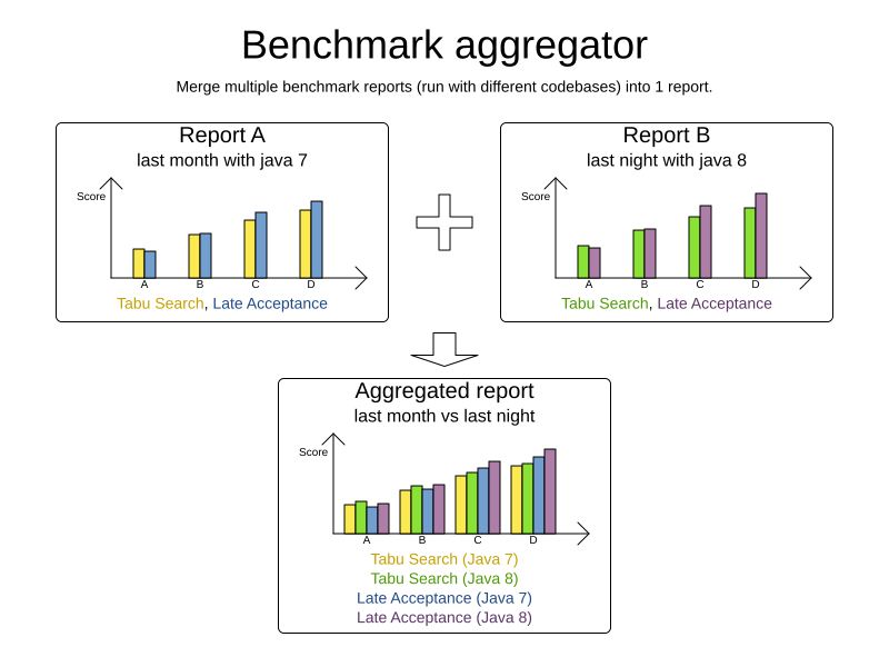
This is useful to:
-
Report on the impact of code changes: Run the same benchmark configuration before and after the code changes, then aggregate a report.
-
Report on the impact of dependency upgrades: Run the same benchmark configuration before and after upgrading the dependency, then aggregate a report.
-
Summarize a too verbose report: Select only the interesting solver benchmarks from the existing report. This especially useful on template reports to make the graphs readable.
-
Partially rerun a benchmark: Rerun part of an existing report (for example only the failed or invalid solvers), then recreate the original intended report with the new values.
Compose the aggregated report in the Benchmark aggregator UI:
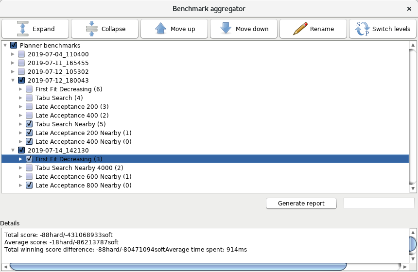
To display that UI, provide a benchmark config to the BenchmarkAggregatorFrame:
    public static void main(String[] args) {
        BenchmarkAggregatorFrame.createAndDisplayFromXmlResource(
                "org/optaplanner/examples/cloudbalancing/benchmark/cloudBalancingBenchmarkConfig.xml");
}|
Despite that it uses a benchmark configuration as input, it ignores all elements of that configuration,
except for the elements |
In the GUI, select the interesting benchmarks and click the button to generate the aggregated report.
|
All the input reports which are being merged should have been generated with the same OptaPlanner version (excluding hotfix differences) as the |